Describe the differences between analog, digital storage, digital phosphor, and digital sampling oscilloscopes
Describe electrical waveform types
Understand basic oscilloscope controls
Take simple measurements
The glossary in the back of this primer will give you definitions of unfamiliar terms. The vocabulary and multiple-choice written exercises on oscilloscope theory and controls make this primer a useful classroom aid. No mathematical or electronics knowledge is necessary.
What are the types of oscilloscopes?
Video Player is loading.
Current Time 0:00
/
Duration 0:00
Loaded: 0%
0:00
Stream Type LIVE
Remaining Time -0:00
1x
Chapters
descriptions off, selected
captions settings, opens captions settings dialog
captions off, selected
This is a modal window.
Beginning of dialog window. Escape will cancel and close the window.
End of dialog window.
This is a modal window. This modal can be closed by pressing the Escape key or activating the close button.
This is a modal window. This modal can be closed by pressing the Escape key or activating the close button.
Video Player is loading.
Current Time 0:00
/
Duration 2:03
Loaded: 8.00%
0:00
Stream Type LIVE
Remaining Time -2:03
1x
Chapters
descriptions off, selected
captions settings, opens captions settings dialog
captions off
English, selected
en (Main), selected
This is a modal window.
Beginning of dialog window. Escape will cancel and close the window.
End of dialog window.
This is a modal window. This modal can be closed by pressing the Escape key or activating the close button.
This is a modal window. This modal can be closed by pressing the Escape key or activating the close button.
Nearly all consumer products today have electronic circuits. Whether a product is simple or complex, if it includes electronic components, the design, verification, and debugging process requires an oscilloscope to analyze the numerous electrical signals that make the product come to life.
Understanding oscilloscope basics is critical to almost all product design.
What exactly is an oscilloscope, anyway? Quite simply, an oscilloscope is a diagnostic instrument that draws a graph of an electrical signal. This simple graph can tell you many things about a signal, such as:
The time and voltage values of a signal.
The frequency of an oscillating signal.
The "moving parts" of a circuit represented by the signal.
The frequency with which a particular portion of the signal occurs relative to other portions.
Whether or not a malfunctioning component is distorting the signal.
How much of a signal is direct current (DC) or alternating current (AC).
How much of the signal is noise and whether the noise is changing with time.
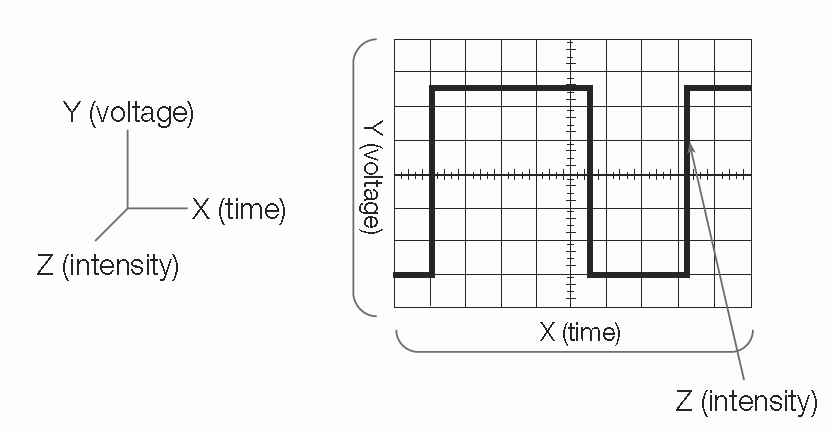
At the most basic level, an oscilloscope's graph of an electrical signal shows how the signal changes over time (Figure 2):
Figure 2: X, Y, and Z components of a displayed waveform.
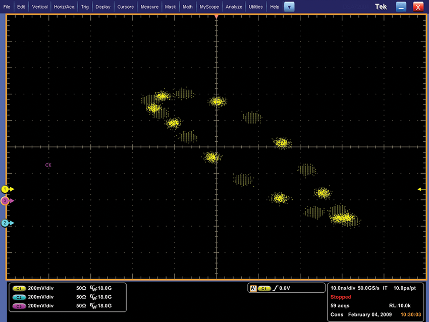
The intensity or brightness of the display is sometimes called the Z-axis. In Digital Phosphor Oscilloscopes (DPO), the Z-axis can be represented by color grading of the display (Figure 3).
Figure 3:Two offset clock patterns with Z axis intensity grading.
The Significance of Signal Integrity
A key benefit of an oscilloscope is its ability to accurately reconstruct a signal. The better the reconstruction of the signal the higher the signal integrity. Here's one way to think of signal integrity. An oscilloscope is analogous to a camera that captures signal images that you then observe and interpret. Several key issues lie at the heart of signal integrity:
When you take a picture, is it an accurate representation of what actually happened?
Is the picture clear or fuzzy?
How many accurate pictures can you take per second?
The different systems and performance capabilities of an oscilloscope contribute to its ability to deliver the highest signal integrity possible. Probes also affect the signal integrity of a measurement system.
This primer helps you understand all of these elements so you can choose and use the oscilloscope appropriate for your application. Before you begin evaluating oscilloscopes, you need to understand the basics of waveforms and waveform measurements.
This information is covered in this chapter. It's the foundation of putting an oscilloscope to work for you.
Understanding Waveforms and Waveform Measurements
The generic term for a pattern that repeats over time is a wave. Sound waves, brain waves, ocean waves, and voltage waves are all repetitive patterns. An oscilloscope measures voltage waves. A waveform is a graphic representation of a wave.
Physical phenomena such as vibrations, temperature, or electrical phenomena such as current or power can be converted to a voltage by a sensor. One cycle of a wave is the portion of the wave that repeats. A voltage waveform shows time on the horizontal axis and voltage on the vertical axis.
Waveform shapes reveal a great deal about a signal. Any time you see a change in the height of the waveform, you know the voltage has changed. Any time there is a flat horizontal line, you know that there is no change for that length of time.
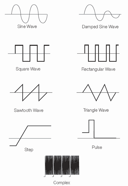
Straight, diagonal lines mean a linear change; a rise or fall of voltage at a steady rate. Sharp angles on a waveform indicate sudden change. Figure 4 shows common waveforms.
Figure 4:Common waveforms
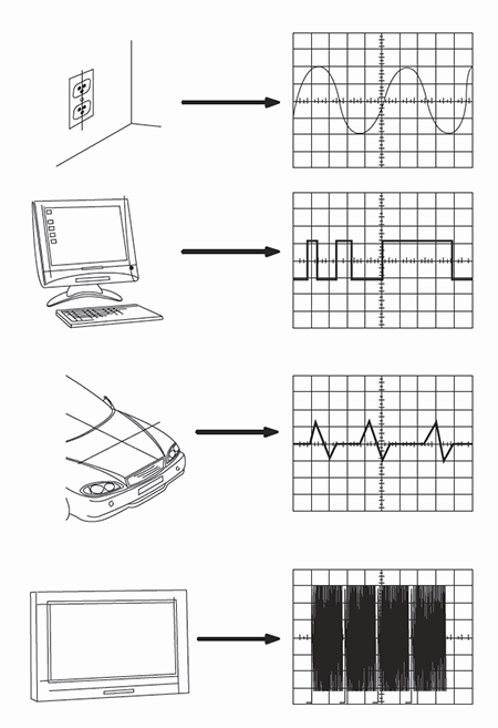
Figure 5 displays sources of common waveforms, such as electrical outlets, computers, automobiles, and televisions.
Figure 5: Sources of common waveforms
Types of Waves
You can classify most waves into these types:
Sine waves.
Square and rectangular waves.
Sawtooth and triangle waves.
Step and pulse shapes.
Periodic and non-periodic signals.
Synchronous and asynchronous signals.
Complex waves.
Next we'll look at each of these types of waves.
Sine Waves
The sine wave is the fundamental wave shape for several reasons. It has harmonious mathematical properties"€it is the same sine shape you may have studied in trigonometry class.
The voltage in a wall outlet varies as a sine wave. Test signals produced by the oscillator circuit of a signal generator are often sine waves.
Most AC power sources produce sine waves (AC signifies alternating current, although the voltage alternates too; DC stands for direct current, which means a steady current and voltage, such as a battery produces.) The damped sine wave is a special case you may see in a circuit that oscillates, but winds down over time.
Square and Rectangular Waves
The square wave is another common wave shape. Basically, a square wave is a voltage that turns on and off (or goes high and low) at regular intervals. It is a standard wave for testing amplifiers. Good amplifiers increase the amplitude of a square wave with minimum distortion.
Television, radio, and computer circuitry often use square waves for timing signals. The rectangular wave is like the square wave except that the high and low time intervals are not of equal length. It is particularly important when analyzing digital circuitry.
Sawtooth and Triangle Waves
Sawtooth and triangle waves result from circuits designed to control voltages linearly, such as the horizontal sweep of an analog oscilloscope or the raster scan of a television.
The transitions between voltage levels of these waves change at a constant rate. These transitions are called ramps.
Step and Pulse Shapes
Signals such as steps and pulses that occur rarely, or non-periodically, are called single-shot or transient signals.
A step indicates a sudden change in voltage, similar to the voltage change you see if you turn on a power switch.
A pulse indicates sudden changes in voltage, similar to the voltage changes you see if you turn a power switch on and then off again. A pulse might represent one bit of information traveling through a computer circuit or it might be a glitch, or defect, in a circuit.
A collection of pulses traveling together creates a pulse train. Digital components in a computer communicate with each other using pulses. These pulses may be in the form of a serial data stream or multiple signal lines may be used to represent a value in a parallel data bus. Pulses are also common in x-ray, radar, and communications equipment.
Periodic and Non-periodic Signals
Repetitive signals are referred to as periodic signals, while signals that constantly change are known as non-periodic signals. A still picture is analogous to a periodic signal, while a movie is analogous to a non-periodic signal.
Synchronous and Asynchronous Signals
When a timing relationship exists between two signals, those signals are referred to as synchronous. Clock, data, and address signals inside a computer are examples of synchronous signals.
Asynchronous signals are signals between which no timing relationship exists. Because no time correlation exists between the act of touching a key on a computer keyboard and the clock inside the computer, these signals are considered asynchronous.
Complex Waves
Some waveforms combine the characteristics of sines, squares, steps, and pulses to produce complex wave shapes. The signal information may be embedded in the form of amplitude, phase, and/or frequency variations.
For example, although the signal in Figure 6 is an ordinary composite video signal, it is composed of many cycles of higher-frequency waveforms embedded in a lower-frequency envelope.
In this example, it is important to understand the relative levels and timing relationships of the steps. To view this signal, you need an oscilloscope that captures the low-frequency envelope and blends in the higher-frequency waves in an intensity-graded fashion so that you can see their overall combination as an image you can interpret visually.
Digital phosphor oscilloscopes (DPOs) are best suited to viewing complex waves, such as the video signals shown in Figure 6. Their displays provide the necessary frequency-of-occurrence information, or intensity grading, that is essential to understanding what the waveform is really doing.
Some oscilloscopes can display certain types of complex waveforms in special ways. For example, telecommunications data may be displayed as an eye pattern or a constellation diagram:
Figure 6: An NTSC composite video signal is an example of a complex wave.
Telecommunications digital data signals can be displayed on an oscilloscope as a special type of waveform referred to as an eye pattern. The name comes from the similarity of the waveform to a series of eyes (Figure 7).
Eye patterns are produced when digital data from a receiver is sampled and applied to the vertical input, while the data rate is used to trigger the horizontal sweep. The eye pattern displays one bit or unit interval of data with all possible edge transitions and states superimposed in one comprehensive view.
Figure 7: 622 Mb/s serial data eye pattern.
A constellation diagram is a representation of a signal modulated by a digital modulation scheme such as quadrature amplitude modulation or phase-shift keying.
Constellation Diagram.
Waveform Measurements
Many terms are used to describe the types of measurements you make with an oscilloscope. Next we'll look at some of the most common measurements and terms.
Frequency and Period
If a signal repeats, it has a frequency. Frequency is measured in Hertz (Hz) and is the number of times the signal repeats itself in one second. This is also referred to as cycles per second.
A repetitive signal also has a period, which is the amount of time it takes the signal to complete one cycle.
Period and frequency are reciprocals of each other, so that:
Figure 8: Frequency and period of a sine wave.
Voltage
Voltage is the amount of electric potential, or signal strength, between two points in a circuit. Usually, one of these points is ground, or zero volts, but not always. You may want to measure the voltage from the maximum peak to the minimum peak of a waveform, referred to as the peak-to-peak voltage.
Amplitude
Amplitude is the amount of voltage between two points in a circuit. Amplitude commonly refers to the maximum voltage of a signal measured from ground, or zero volts. The waveform shown in Figure 9 has an amplitude of 1 V and a peak-to-peak voltage of 2 V.
Figure 9: Amplitude and degrees of a sine wave.
Phase
Phase is best explained by looking at a sine wave. The voltage level of sine waves is based on circular motion. Given that a circle has 360°, one cycle of a sine wave has 360°, as shown in Figure 10.
Using degrees, you can refer to the phase angle of a sine wave when you want to describe how much of the period has elapsed.
Phase shift describes the difference in timing between two otherwise similar signals. The waveform in Figure 10 labeled "current" is said to be 90° out of phase with the waveform labeled "voltage," since the waves reach similar points in their cycles exactly 1/4 of a cycle apart (360°/4 = 90°). Phase shifts are common in electronics.
Figure 10: Phase shift.
Waveform Measurements with Digital Oscilloscopes
Digital oscilloscopes have functions that make waveform measurements easy. They have front-panel buttons and screen-based menus from which you can select fully-automated measurements. These include amplitude, period, rise/fall time, and many more.
Many digital oscilloscopes also provide mean and RMS calculations, duty cycle, and other math operations. Automated measurements appear as on-screen alphanumeric readouts. Typically these readings are more accurate than is possible to obtain with direct graticule interpretation.
Oscilloscope Types Explained: Analog vs. Digital Functionality
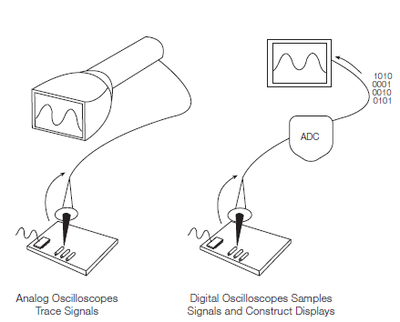
Electronic equipment can be classified into two categories: analog and digital. Analog equipment works with continuously variable voltages, while digital equipment works with discrete binary numbers that represent voltage samples. A conventional phonograph is an analog device, while a CD player is a digital device. Oscilloscopes can be classified similarly – as analog and digital types. In contrast to an analog oscilloscope, a digital oscilloscope uses an analog-to-digital converter (ADC) to convert the measured voltage into digital information. It acquires the waveform as a series of samples, and stores these samples until it accumulates enough samples to describe a waveform. The digital oscilloscope then reassembles the waveform for display on the screen, as shown in Figure 11.
Figure 11: Analog oscilloscopes trace signals, while digital oscilloscopes sample signals and construct displays.
Types of Digital Oscilloscopes
Digital oscilloscopes can be classified into four types:
Digital storage oscilloscopes (DSO)
Digital phosphor oscilloscopes (DPO)
Mixed signal oscilloscopes (MSO)
Digital sampling oscilloscopes
This chapter describes these types of digital oscilloscopes in detail to help you zero in on the type of oscilloscope that’s right for your needs.
Digital Storage Oscilloscopes (DSO)
A conventional digital oscilloscope is known as a digital storage oscilloscope (DSO). Its display typically relies on a raster-type screen rather than the luminous phosphor found in older analog oscilloscopes.
DSOs allow you to capture and view events that may happen only once, known as transients. Because the waveform information exists in digital form as a series of stored binary values, it can be analyzed, archived, printed, and otherwise processed, within the oscilloscope itself or by an external computer.
The waveform need not be continuous; it can be displayed even when the signal disappears. Unlike analog oscilloscopes, DSOs provide permanent signal storage and extensive waveform processing. However, DSOs typically have no real-time intensity grading. Therefore they cannot express varying levels of intensity in the live signal.
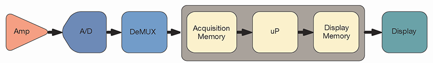
Some of the subsystems in DSOs are similar to those in analog oscilloscopes. However, DSOs contain additional data-processing subsystems that are used to collect and display data for the entire waveform. A DSO employs a serial-processing architecture to capture and display a signal on its screen, as shown in Figure 12.
Figure 12: The serial-processing architecture of a digital storage oscilloscope (DSO).
Serial-processing Architecture
Like an analog oscilloscope, a DSO’s first (input) stage is a vertical amplifier. Vertical controls allow you to adjust the amplitude and position range at this stage. Next, the analog to digital converter (ADC) in the horizontal system samples the signal at discrete points in time and converts the signal’s voltage at these points into digital values called sample points. This process is referred to as digitizing a signal.
The horizontal system’s sample clock determines how often the ADC takes a sample. This rate is referred to as the sample rate and is expressed in samples per second (S/s).
The sample points from the ADC are stored in acquisition memory as waveform points. Several sample points may comprise one waveform point. Together, the waveform points comprise one waveform record. The number of waveform points used to create a waveform record is called the record length. The trigger system determines the start and stop points of the record.
The DSO’s signal path includes a microprocessor through which the measured signal passes on its way to the display. This microprocessor processes the signal, coordinates display activities, manages the front panel controls, and more. The signal then passes through the display memory and is displayed on the oscilloscope screen.
Depending on the capabilities of an oscilloscope, additional processing of the sample points may take place, which enhances the display. Pre-trigger may also be available so you can see events before the trigger point. Most digital oscilloscopes also provide a selection of automatic parametric measurements, simplifying the measurement process.
DSOs provide high performance in a single-shot, multi-channel instrument (Figure 13). They are ideal for low repetition-rate or single-shot, high-speed, multichannel design applications. In the real world of digital design, an engineer usually examines four or more signals simultaneously, making the DSO a critical companion.
Figure 13: The digital storage oscilloscope delivers high-speed, single-shot acquisition across multiple channels, increasing the likelihood of capturing elusive glitches and transient events
Digital Phosphor Oscilloscopes (DPO)
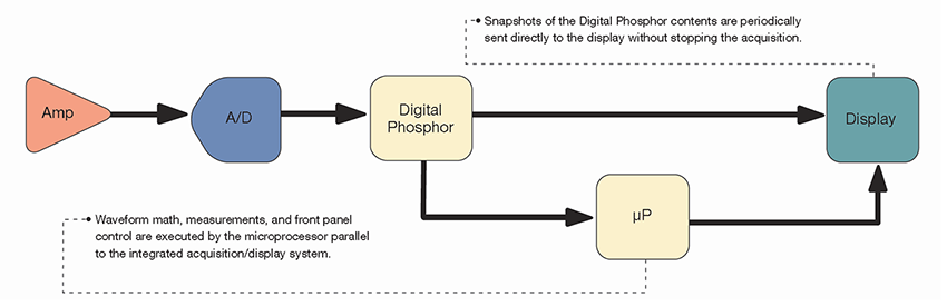
The digital phosphor oscilloscope (DPO) offers a new approach to oscilloscope architecture. This architecture enables it to deliver unique acquisition and display capabilities to accurately reconstruct a signal. While a DSO uses a serial-processing architecture to capture, display, and analyze signals, a DPO employs a parallel processing architecture to perform these functions (Figure 14).
Figure 14: The parallel-processing architecture of a digital phosphor oscilloscope (DPO).
The DPO architecture dedicates unique ASIC hardware to acquire waveform images, delivering high waveform capture rates, resulting in a higher level of signal visualization. This performance increases the probability of witnessing transient events that occur in digital systems, such as runt pulses, glitches and transition errors, and enables additional analysis capability.
Parallel-processing Architecture
A DPO’s first (input) stage is similar to that of an analog oscilloscope—a vertical amplifier—and its second stage is similar to that of a DSO—an ADC. But, the DPO differs significantly from its predecessors following the analog-to-digital conversion.
For any oscilloscope—analog, DSO, or DPO—there is always a hold-off time during which the instrument processes the most recently acquired data, resets the system, and waits for the next trigger event. During this time, the oscilloscope is blind to all signal activity. The probability of seeing an infrequent or low repetition event decreases as the hold off time increases.
It is impossible to determine the probability of capture by simply looking at the display update rate. If you rely solely on the update rate, it is easy to make the mistake of believing that the oscilloscope is capturing all pertinent information about the waveform when, in fact, it is not.
The DSO processes captured waveforms serially. The speed of its microprocessor is a bottleneck in this process because it limits the waveform capture rate. The DPO rasterizes the digitized waveform data into a digital phosphor database. Every 1/30th of a second—about as fast as the human eye can perceive it—a snapshot of the signal image that is stored in the database is pipelined directly to the display. This direct rasterization of waveform data, and direct copy to display memory from the database, removes the data-processing bottleneck inherent in other architectures. The result is an enhanced “real-time” and lively display update. Signal details, intermittent events, and dynamic characteristics of the signal are captured in real-time. The DPO’s microprocessor works in parallel with this integrated acquisition system for display management, measurement automation, and instrument control, so that it does not affect the oscilloscope’s acquisition speed.
A DPO faithfully emulates the best display attributes of an analog oscilloscope, displaying the signal in three dimensions: time, amplitude, and the distribution of amplitude over time. All in real-time.
Unlike an analog oscilloscope’s reliance on chemical phosphor, a DPO uses a purely electronic digital phosphor that’s actually a continuously updated database. This database has a separate “cell” of information for every single pixel in the oscilloscope’s display. Each time a waveform is captured—in other words, every time the oscilloscope triggers—it is mapped into the digital phosphor database’s cells. Each cell that represents a screen location and is touched by the waveform is reinforced with intensity information, while other cells are not. Thus, intensity information builds up in cells where the waveform passes most often.
When the digital phosphor database is fed to the oscilloscope’s display, the display reveals intensified waveform areas, in proportion to the signal’s frequency of occurrence at each point, much like the intensity grading characteristics of an analog oscilloscope. The DPO also allows the display of the varying frequency-of-occurrence information on the display as contrasting colors, unlike an analog oscilloscope. With a DPO, it is easy to see the difference between a waveform that occurs on almost every trigger and one that occurs, say, every 100th trigger.
A DPO break down the barrier between analog and digital oscilloscope technologies. They are equally suitable for viewing high and low frequencies, repetitive waveforms, transients, and signal variations in real-time. Only a DPO provides the Z-axis (intensity) in real-time that is missing from conventional DSOs.
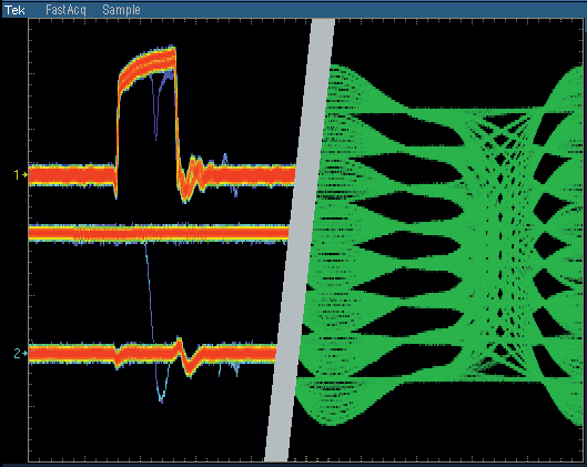
A DPO is ideal for those who need the best general purpose design and troubleshooting tool for a wide range of applications (Figure 15). A DPO is exemplary for advanced analysis, communication mask testing, digital debug of intermittent signals, repetitive digital design. and timing applications.
Figure 15: Some DPOs can acquire millions of waveform in just seconds, significantly increasing the probability of capturing intermittent and elusive events and revealing dynamic signal behavior.
Mixed Domain Oscilloscopes (MDO)
Electronic equipment can be classified into two categories: analog and digital. Analog equipment works with continuously variable voltages, while digital equipment works with discrete binary numbers that represent voltage samples. A phonograph is an analog device, while an MP3 player is a digital device.
Figure 16: Time-correlated display of a Zigbee radio's microprocessor SPI (MOSI) and (MISO) control lines, with measurements of drain current and voltage to the radio IC and the spectrum during turn-on.
Mixed Signal Oscilloscopes (MSO)
The mixed signal oscilloscope (MSO) combines the performance of a DPO with the basic functionality of a 16-channel logic analyzer, including parallel/serial bus protocol decoding and triggering.
The MSO's digital channels view a digital signal as either a logic high or logic low, just like a digital circuit views the signal. This means as long as ringing, overshoot and ground bounce do not cause logic transitions, these analog characteristics are not of concern to the MSO. Just like a logic analyzer, a MSO uses a threshold voltage to determine if the signal is logic high or logic low.
The MSO is the tool of choice for quickly debugging digital circuits using its powerful digital triggering, high-resolution acquisition capability, and analysis tools. The root cause of many digital problems is quicker to pinpoint by analyzing both the analog and digital representations of the signal, as shown in Figure 17, making an MSO ideal for verifying and debugging digital circuits.
Figure 17: The MSO provides 16 integrated digital channels, enabling the ability to view and analyze time-correlated analog and digital signals.
Digital Sampling Oscilloscopes
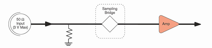
In contrast to the digital storage and DPO architectures, the architecture of the digital sampling oscilloscope reverses the position of the attenuator/ amplifier and the sampling bridge (Figure 18). The input signal is sampled before any attenuation or amplification is performed. A low bandwidth amplifier can then be used after the sampling bridge because the signal has already been converted to a lower frequency by the sampling gate, resulting in a much higher bandwidth instrument.
Figure 18: The parallel-processing architecture of a digital phosphor oscilloscope (DPO).
The tradeoff for this high bandwidth, however, is that the sampling oscilloscope’s dynamic range is limited. Since there is no attenuator/amplifier in front of the sampling gate, there is no facility to scale the input. The sampling bridge must be able to handle the full dynamic range of the input at all times. Therefore, the dynamic range of most sampling oscilloscopes is limited to about 1 V peak-to-peak. Digital storage and DPOs, on the other hand, can handle 50 to 100 volts.
In addition, protection diodes cannot be placed in front of the sampling bridge, as this limits the bandwidth. This reduces the safe input voltage for a sampling oscilloscope to about 3 V, as compared to 500 V available on other oscilloscopes.
When measuring high-frequency signals, the DSO or DPO may not be able to collect enough samples in one sweep. A digital sampling oscilloscope is an ideal tool for accurately capturing signals whose frequency components are much higher than the oscilloscope’s sample rate (Figure 19). This oscilloscope is capable of measuring signals of up to an order of magnitude faster than any other oscilloscope. It can achieve bandwidth and high-speed timing ten times higher than other oscilloscopes for repetitive signals. Sequential equivalent-time sampling oscilloscopes are available with bandwidths to 80 GHz.
Figure 19: Time domain reflectometry (TDR) display from a digital sampling oscilloscope.
Evaluating Oscilloscopes: Learn About Key Features & Functions
Once you've determined the type of oscilloscope you need, there are still many models to choose from, including portable and hand-held. And when choosing an oscilloscope, there are a number of things to consider, such as the ease-of use, sample rate the probes used to bring data into it, and all the elements of an oscilloscope that affect its ability to achieve the required signal integrity.
To understand these considerations, we'll look briefly at ease-of-use and probes, and then describe some useful measurement and oscilloscope performance terms. These terms cover the criteria essential to choosing the right oscilloscope for your application.
Ease-of-Use
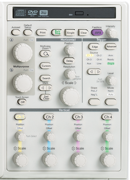
Oscilloscopes should be easy to learn and easy to use, helping you work at peak efficiency and productivity. This means you can focus on your design, rather than the measurement tools. Just as there is no one typical car driver, there is no one typical oscilloscope user. Regardless of whether you prefer a traditional instrument interface or a Windows® software interface, it is important to have flexibility in your oscilloscope's operation. Many oscilloscopes offer a balance between performance and simplicity by providing many ways to operate the instrument. A typical oscilloscope's front-panel layout (Figure 60) provides dedicated vertical, horizontal and trigger controls.
Figure 60: Traditional, analog-style knobs control position, scale, intensity, etc. – precisely as you would expect.
The Complete Measurement System Probes
Even the most advanced instrument can only be as precise as the data that goes into it. A probe works in conjunction with an oscilloscope as part of the measurement system. Precision measurements start at the probe tip. The right probes matched to the oscilloscope and the device under test (DUT) not only allow the signal to be brought to the oscilloscope cleanly, they also amplify and preserve the signal for the greatest signal integrity and measurement accuracy. Please refer to the Tektronix ABCs of Probes Primer for more information about probes and probe accessories.
Bandwidth
Bandwidth determines an oscilloscope's fundamental ability to measure a signal. As signal frequency increases, the capability of an oscilloscope to accurately display the signal decreases. The bandwidth specification indicates the frequency range that the oscilloscope can accurately measure.
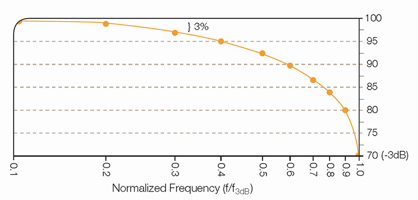
Oscilloscope bandwidth is specified as the frequency at which a sinusoidal input signal is attenuated to 70.7% of the signal's true amplitude, known as the –3 dB point, a term based on a logarithmic scale, as shown in Figure 44.
Figure 44: Oscilloscope bandwidth is the frequency at which a sinusoidal input signal is attenuated to 70.7% of the signal's true amplitude, known as the -3 dB point.
Without adequate bandwidth, an oscilloscope cannot resolve high-frequency changes. Amplitude is distorted. Edges vanish. Details are lost. All the features, bells and whistles in your oscilloscope will mean nothing.
To determine the oscilloscope bandwidth needed to accurately characterize signal amplitude in your specific application, apply the “5 Times Rule”:
5 Times Rule
An oscilloscope selected using the “5 Times Rule” provides less than ±2% error in your measurements. This is typically sufficient for today's applications. However, as signal speeds increase, it may not be possible to achieve this rule of thumb. Keep in mind that higher bandwidth will likely provide more accurate reproduction of a signal, as shown in Figure 45.
Figure 45: The higher the bandwidth, the more accurate the reproduction of your signal, as illustrated with a signal captured at 250 MHz, 1 GHz and 4 GHz bandwidth levels.
Some oscilloscopes provide a method of enhancing the bandwidth through digital signal processing (DSP). A DSP arbitrary equalization filter can be used to improve the oscilloscope channel response. This filter extends the bandwidth, flattens the oscilloscope's channel frequency response, improves phase linearity, and provides a better match between channels. It also decreases rise time and improves the time domain step response.
Rise Time
Rise time describes the useful frequency range of an oscilloscope. Rise time measurements are critical in the digital world. Rise time may be a more appropriate performance consideration when you expect to measure digital signals, such as pulses and steps. An oscilloscope must have sufficient rise time to accurately capture the details of rapid transitions (Figure 46).
Figure 46: Rise time characterization of a high-speed digital signal.
To calculate the oscilloscope rise time required for your signal type, use this equation:
Oscilloscope Rise Time
Using this equation is similar to using the equation for bandwidth. As in the case of bandwidth, achieving this rule of thumb may not always be possible given the extreme speeds of today's signals. Always remember that an oscilloscope with faster rise time will more accurately capture the critical details of fast transitions.
In some applications, you may know only the rise time of a signal. A constant allows you to relate the bandwidth and rise time of the oscilloscope using this equation:
Bandwidth and Rise Time
Where K is a value between 0.35 and 0.45, depending on the shape of the oscilloscope's frequency response curve and pulse rise time response. Oscilloscopes with a bandwidth of <1 GHz typically have a 0.35 value, while oscilloscopes with a bandwidth of> 1 GHz usually have a value between 0.40 and 0.45.
Some logic families produce inherently faster rise times than others (Figure 47).
Figure 47: Some logic families produce inherently faster rise times than others.
Sample Rate
Sample rate is specified in samples per second (S/s). It defines how frequently a digital oscilloscope takes a snapshot or sample of the signal, analogous to the frames in a movie. The faster an oscilloscope samples (i.e., the higher the sample rate), the greater the resolution and detail of the displayed waveform and the less likely that critical information or events is lost (Figure 48).
Figure 48: A higher sample rate provides greater signal resolution, ensuring that you'll see intermittent events.
The minimum sample rate may also be important if you need to look at slowly changing signals over longer periods of time. Typically, the displayed sample rate changes with changes made to the horizontal scale control to maintain a constant number of waveform points in the displayed waveform record.
How do you calculate your sample rate requirements? The method differs based on the type of waveform you are measuring, and the method of signal reconstruction used by the oscilloscope.
In order to accurately reconstruct a signal and avoid aliasing, the Nyquist theorem states that the signal must be sampled at least twice as fast as its highest frequency component. This theorem, however, assumes an infinite record length and a continuous signal. Since no oscilloscope offers infinite record length and, by definition, glitches are not continuous, sampling at only twice the rate of highest frequency component is usually insufficient.
In reality, accurate reconstruction of a signal depends on both the sample rate and the interpolation method used to fill in the spaces between the samples. Some oscilloscopes let you select either sin (x)/x interpolation for measuring sinusoidal signals, or linear interpolation for square waves, pulses and other signal types.
For accurate reconstruction using sin (x)/x interpolation, your oscilloscope should have a sample rate at least 2.5 times the highest frequency component of your signal. Using linear interpolation, the sample rate should be at least 10 times the highest frequency signal component.
Some measurement systems with sample rates to 10 GS/s and bandwidths to 3+ GHz are optimized for capturing very fast, single-shot and transient events by oversampling up to 5 times the bandwidth.
A Note About Bandwidth and Sample Rate
The digital approach means that the oscilloscope can display any frequency within its range with stability, brightness, and clarity. For repetitive signals, the bandwidth of the digital oscilloscope is a function of the analog bandwidth of the front-end components of the oscilloscope, commonly referred to as the –3 dB point. For single-shot and transient events, such as pulses and steps, the bandwidth can be limited by the oscilloscope's sample rate.
Waveform Capture Rate
All oscilloscopes blink. That is, they open their eyes a given number of times per second to capture the signal, and close their eyes in between. This is the waveform capture rate, expressed as waveforms per second (wfms/s). While the sample rate indicates how frequently the oscilloscope samples the input signal within one waveform, or cycle, the waveform capture rate refers to how quickly an oscilloscope acquires waveforms.
Waveform capture rates vary greatly, depending on the type and performance level of the oscilloscope. Oscilloscopes with high waveform capture rates provide significantly more visual insight into signal behavior, and dramatically increase the probability that the oscilloscope will quickly capture transient anomalies such as jitter, runt pulses, glitches and transition errors.
Digital storage oscilloscopes (DSO) employ a serial processing architecture to capture from 10 to 5,000 wfms/s. Some DSOs provide a special mode that bursts multiple captures into long memory, temporarily delivering higher waveform capture rates followed by long processing dead times that reduce the probability of capturing rare, intermittent events.
Most digital phosphor oscilloscopes (DPO) employ a parallel processing architecture to deliver vastly greater waveform capture rates. Some DPOs can acquire millions of waveforms in just seconds, significantly increasing the probability of capturing intermittent and elusive events and allowing you to see the problems in your signal more quickly (Figure 49).
Figure 49: A DPO provides an ideal solution for non-repetitive, high-speed, multi-channel digital design applications.
Moreover, the DPO's ability to acquire and display three dimensions of signal behavior in real time—amplitude, time and distribution of amplitude over time—results in a superior level of insight into signal behavior (Figure 50).
Figure 50: A DPO enables a superior level of insight into signal behavior by - delivering vastly greater waveform capture rates and three-dimensional - display, making it the best general-purpose design and troubleshooting - tool for a wide range of applications.
Record Length
Record length, expressed as the number of points that comprise a complete waveform record, determines the amount of data that can be captured with each channel. Since an oscilloscope can store only a limited number of samples, the waveform duration (time) is inversely proportional to the oscilloscope's sample rate:
Time Interval
Oscilloscopes allow you to select record length to optimize the level of detail needed for your application. If you are analyzing an extremely stable sinusoidal signal, you may need only a 500 point record length, but if you are isolating the causes of timing anomalies in a complex digital data stream, you may need a million points or more for a given record length, as shown in Figure 51.
Figure 51: Capturing the high frequency detail of this modulated 85 MHz carrier requires high resolution sampling (100 ps). Seeing the signal's complete modulation envelope requires a long time duration (1 ms). Using long record length (10 MB), the oscilloscope can display both.
Triggering Capabilities
An oscilloscope's trigger function synchronizes the horizontal sweep at the correct point of the signal. This is essential for clear signal characterization. Trigger controls allow you to stabilize repetitive waveforms and capture single-shot waveforms.
Effective Bits
Effective bits represent a measure of a digital oscilloscope's ability to accurately reconstruct a sine wave signal's shape. This measurement compares the oscilloscope's actual error to that of a theoretical “ideal” digitizer. Because the actual errors include noise and distortion, the frequency and amplitude of the signal must be specified.
Frequency Response
Bandwidth alone is not enough to ensure that an oscilloscope can accurately capture a high frequency signal. The goal of oscilloscope design is a specific type of frequency response: maximally flat envelope delay (MFED). A frequency response of this type delivers excellent pulse fidelity with minimum overshoot and ringing. Since a digital oscilloscope is composed of real amplifiers, attenuators, ADCs, interconnects, and relays, MFED response is a goal that can only be approached. Pulse fidelity varies considerably with model and manufacturer.
Vertical Sensitivity
Vertical sensitivity indicates how much the vertical amplifier can amplify a weak signal. This is usually measured in millivolts (mV) per division. The smallest voltage detected by a general-purpose oscilloscope is typically about 1 mV per vertical screen division.
Sweep Speed
Sweep speed indicates how fast the trace can sweep across the oscilloscope screen, making it possible to see fine details. The sweep speed of an oscilloscope is represented by time (seconds) per division.
Gain Accuracy
Gain accuracy indicates how accurately the vertical system attenuates or amplifies a signal, usually represented as a percentage error.
Horizontal Accuracy (Time Base)
Horizontal accuracy, or time base accuracy, indicates how accurately the horizontal system displays the timing of a signal, usually represented as a percentage error.
Vertical Resolution (Analog-to-Digital Converter)
Vertical resolution of the analog-to-digital converter (ADC), and therefore, the digital oscilloscope, indicates how precisely it can convert input voltages into digital values. Vertical resolution is measured in bits. Calculation techniques can improve the effective resolution, as exemplified with hi-res acquisition mode.
Timing Resolution Mixed Signal Oscilloscopes (MSO)
An important MSO acquisition specification is the timing resolution used for capturing digital signals. Acquiring a signal with better timing resolution provides a more accurate timing measurement of when the signal changes. For example, a 500 MS/s acquisition rate has 2 ns timing resolution and the acquired signal edge uncertainty is 2 ns. A smaller timing resolution of 60.6 ps (16.5 GS/s) decreases the signal edge uncertainty to 60.6 ps and captures faster changing signals.
Some MSOs internally acquire digital signals with two types of acquisitions at the same time. The first acquisition is with standard timing resolution, and the second acquisition uses a high-speed resolution. The standard resolution is used over a longer record length while the high-speed timing acquisition offers more resolution around a narrow point of interest (Figure 52).
Figure 52: The MSO provides 16 integrated digital channels, enabling the ability to view and analyze time-correlated analog and digital signals. A high speed timing acquisition provides more resolution to reveal narrow events such as glitches.
Connectivity
The need to analyze measurement results remains of utmost importance. The need to document and share information and measurement results easily and frequently has also grown in importance. The connectivity of an oscilloscope delivers advanced analysis capabilities and simplifies the documentation and sharing of results. As shown in Figure 53, standard interfaces (GPIB, RS-232, USB, and Ethernet) and network communication modules enable some oscilloscopes to deliver a vast array of functionality and control.
Figure 53: Today's oscilloscopes provide a wide array of communications interfaces, such as a standard Centronics port and optional Ethernet/RS-232, GPIB/RS-232, and VGA/RS-232 modules. There is even a USB port (not shown) on the front panel.
Some advanced oscilloscopes also let you:
Create, edit and share documents on the oscilloscope, all while working with the instrument in your particular environment
Access network printing and file sharing resources
Access the Windows® desktop
Run third-party analysis and documentation software
Link to networks
Access the Internet
Send and receive e-mail
Expandability
An oscilloscope should be able to accommodate your needs as they change. Some oscilloscopes allow you to:
Add memory to channels to analyze longer record lengths
Add application-specific measurement capabilities
Complement the power of the oscilloscope with a full range of probes and modules
Work with popular third-party analysis and productivity
Windows-compatible software
Add accessories, such as battery packs and rack mounts
Application modules and software may enable you to transform your oscilloscope into a highly-specialized analysis tool capable of performing functions such as jitter and timing analysis, microprocessor memory system verification, communications standards testing, disk drive measurements, video measurements, power measurements and much more. Figures 54 through 59 highlight a few of these examples.
Figure 54: Analysis software packages are specifically designed to meet jitter and eye measurement needs of today's high-speed digital designers.
Figure 55: Serial bus analysis is accelerated with automated trigger, decode, and search on serial packet context.
Figure 57: Advanced DDR analysis tools automate complex memory tasks like separating read/write bursts and performing JEDEC measurements.
Figure 58: Video application modules make the oscilloscope a fast, tell-all tool for video troubleshooting.
Figure 59: Advanced analysis and productivity software, such as MATLAB®, can be installed in Windows-based oscilloscopes to accomplish local signal analysis.
Oscilloscope Systems and Controls: Vertical, Horizontal & Triggering Explained
Analog and digital oscilloscopes have some basic controls that are similar, and some that are different. We’ll look at the basic systems and controls that are common to both. Understanding these systems and controls is key to using an oscilloscope to tackle your specific measurement challenges. Note that your oscilloscope probably has additional controls not discussed here.
The Three Systems
A basic oscilloscope consists of three different systems – the vertical system, horizontal system, and trigger system. Each system contributes to the oscilloscope’s ability to accurately reconstruct a signal.
The front panel of an oscilloscope is divided into three sections labeled Vertical, Horizontal, and Trigger. Your oscilloscope may have other sections, depending on the model and type.
When using an oscilloscope, you adjust settings in these areas to accommodate an incoming signal:
Vertical: This is the attenuation or amplification of the signal. Use the volts/div control to adjust the amplitude of the signal to the desired measurement range.
Horizontal: This is the time base. Use the sec/div control to set the amount of time per division represented horizontally across the screen.
Trigger: This is the triggering of the oscilloscope. Use the trigger level to stabilize a repeating signal, or to trigger on a single event.
We’ll look at each of these systems and controls, in this chapter.
Figure 20: Front-panel control section of an oscilloscope.
Vertical System and Controls
Vertical controls are used to position and scale the waveform vertically, set the input coupling, and adjust other signal conditioning. Common vertical controls include:
Position
Coupling: DC, AC, and GND
Bandwidth: Limit and Enhancement
Termination: 1M ohm and 50 ohm
Offset
Invert: On/Off
Scale: Fixed Steps and Variable
Some of these controls are described next.
Position and Volts per Division
The vertical position control allows you to move the waveform up and down so it’s exactly where you want it on the screen.
The volts-per-division setting (usually written as volts/div) is a scaling factor that varies the size of the waveform on the screen. If the volts/div setting is 5 volts, then each of the eight vertical divisions represents 5 volts and the entire screen can display 40 volts from bottom to top, assuming a graticule with eight major divisions. If the setting is 0.5 volts/div, the screen can display 4 volts from bottom to top, and so on.
The maximum voltage you can display on the screen is the volts/div setting multiplied by the number of vertical divisions. Note that the probe you use, 1X or 10X, also influences the scale factor.
You must divide the volts/div scale by the attenuation factor of the probe if the oscilloscope does not do it for you. Often the volts/div scale has either a variable gain or a fine gain control for scaling a displayed signal to a certain number of divisions. Use this control to assist in taking rise time measurements.
Input Coupling
Coupling refers to the method used to connect an electrical signal from one circuit to another. In this case, the input coupling is the connection from your test circuit to the oscilloscope.
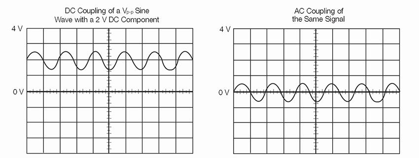
The coupling can be set to DC, AC, or ground. DC coupling shows all of an input signal. AC coupling blocks the DC component of a signal so that you see the waveform centered around zero volts. Figure 21 illustrates this difference.
The AC coupling setting is useful when the entire signal (alternating current + direct current) is too large for the volts/div setting.
Figure 21: AC and DC input coupling.
The ground setting disconnects the input signal from the vertical system, which lets you see where zero volts is located on the screen.
With grounded input coupling and auto trigger mode, you see a horizontal line on the screen that represents zero volts. Switching from DC to ground and back again is a handy way of measuring signal voltage levels with respect to ground.
Bandwidth Limit
Most oscilloscopes have a circuit that limits the bandwidth of the oscilloscope. By limiting the bandwidth, you reduce the noise that sometimes appears on the displayed waveform, resulting in a cleaner signal display.
Note that while eliminating noise, the bandwidth limit can also reduce or eliminate high frequency signal content.
Bandwidth Enhancement
Some oscilloscopes may provide a DSP arbitrary equalization filter that can be used to improve the oscilloscope channel response. This filter extends the bandwidth, flattens the oscilloscope channel frequency response, improves phase linearity, and provides a better match between channels. It also decreases rise time and improves the time domain step response.
Horizontal System and Controls
An oscilloscope’s horizontal system is most closely associated with its acquisition of an input signal. Sample rate and record length are among the considerations here. Horizontal controls are used to position and scale the waveform horizontally. Common horizontal controls include:
Acquisition
Sample Rate
Position and Seconds per Division
Time Base
Zoom/Pan
Search
XY Mode
Z Axis
XYZ Mode
Trigger Position
Scale
Trace Separation
Record Length
Resolution
Some of these controls are described next.
Acquisition Controls
Digital oscilloscopes have settings that let you control how the acquisition system processes a signal. Figure 22 shows an example of an acquisition menu.
Look over the acquisition options on your digital oscilloscope while you read this section.
Figure 22: Example of an acquisition menu.
Acquisition Modes
Acquisition modes control how waveform points are produced from sample points. Sample points are the digital values derived directly from the analog-to-digital converter (ADC). The sample interval refers to the time between these sample points.
Waveform points are the digital values that are stored in memory and displayed to construct the waveform. The time-value difference between waveform points is referred to as the waveform interval.
The sample interval and the waveform interval may or may not be the same. This fact leads to the existence of several different acquisition modes in which one waveform point is comprised of several sequentially acquired sample points.
Additionally, waveform points can be created from a composite of sample points taken from multiple acquisitions, which provides another set of acquisition modes. A description of the most commonly used acquisition modes follows.
Sample Mode: This is the simplest acquisition mode. The oscilloscope creates a waveform point by saving one sample point during each waveform interval.
Peak Detect Mode: The oscilloscope saves the minimum and maximum value sample points taken during two waveform intervals and uses these samples as the two corresponding waveform points.
Digital oscilloscopes with peak detect mode run the ADC at a fast sample rate, even at very slow time base settings (slow time base settings translate into long waveform intervals) and are able to capture fast signal changes that would occur between the waveform points if in sample mode (Figure 23).
Figure 23: Sample rate varies with time base settings - the slower the time based setting, the slower the sample rate. Some digital oscilloscopes provide peak detect mode to capture fast transients at slow sweep speeds.
Peak detect mode is particularly useful for seeing narrow pulses spaced far apart in time, as shown in Figure 24.
Figure 24: Advanced analysis and productivity software, such as MATLAB®, can be installed in Windows-based oscilloscopes to accomplish local signal analysis.
Hi-Res Mode: Like peak detect, hi-res mode is a way of getting more information in cases when the ADC can sample faster than the time base setting requires. In this case, multiple samples taken within one waveform interval are averaged together to produce one waveform point.
The result is a decrease in noise and an improvement in resolution for low-speed signals. The advantage of Hi-Res Mode over Average is that Hi-Res Mode can be used even on a single shot event.
Envelope Mode: Envelope mode is similar to peak detect mode. However, in envelope mode, the minimum and maximum waveform points from multiple acquisitions are combined to form a waveform that shows min/max accumulation over time.
Peak detect mode is usually used to acquire the records that are combined to form the envelope waveform.
Average Mode: In average mode, the oscilloscope saves one sample point during each waveform interval as in sample mode. However, waveform points from consecutive acquisitions are then averaged together to produce the final displayed waveform.
Average mode reduces noise without loss of bandwidth, but requires a repeating signal.
Waveform Database Mode: In waveform database mode, the oscilloscope accumulates a waveform database that provides a three-dimensional array of amplitude, time, and counts.
Starting and Stopping the Acquisition System
One of the greatest advantages of digital oscilloscopes is their ability to store waveforms for later viewing.
To this end, there are usually one or more buttons on the front panel that allow you to start and stop the acquisition system so you can analyze waveforms at your leisure.
Additionally, you may want the oscilloscope to automatically stop acquiring after one acquisition is complete or after one set of records has been turned into an envelope or average waveform.
This feature is commonly called single sweep or single sequence and its controls are usually found either with the other acquisition controls or with the trigger controls.
Sampling
Sampling is the process of converting a portion of an input signal into a number of discrete electrical values for the purpose of storage, processing, and/or display. The magnitude of each sampled point is equal to the amplitude of the input signal at the instant in time in which the signal is sampled.
Sampling is like taking snapshots. Each snapshot corresponds to a specific point in time on the waveform. These snapshots can then be arranged in the appropriate order in time to reconstruct the input signal.
In a digital oscilloscope, an array of sampled points is reconstructed on a display with the measured amplitude on the vertical axis and time on the horizontal axis (Figure 25).
The input waveform in Figure 25 appears as a series of dots on the screen. If the dots are widely spaced and difficult to interpret as a waveform, the dots can be connected using a process called interpolation.
Interpolation connects the dots with lines or vectors. A number of interpolation methods are available that can be used to produce an accurate representation of a continuous input signal.
Figure 25: Basic sampling, showing sample points are connected by interpolation to produce a continuous waveform.
Sampling Controls
Some digital oscilloscopes provide you with a choice in sampling method, either real-time sampling or equivalent time sampling. The acquisition controls available with these oscilloscopes allow you to select a sample method to acquire signals.
Note that this choice makes no difference for slow time base settings and only has an effect when the ADC cannot sample fast enough to fill the record with waveform points in one pass. Each sampling method has distinct advantages, depending on the kind of measurements being made.
Controls are typically available to give you the choice of three horizontal time base modes of operations. If you are simply doing signal exploration and want to interact with a lively signal, you use the Automatic or Interactive Default mode that provides you with the liveliest display update rate.
If you want a precise measurement and the highest real-time sample rate that will give you the most measurement accuracy, then you use the Constant Sample Rate mode. It maintains the highest sample rate and provides the best real-time resolution.
The last mode is called the Manual mode because it ensures direct and independent control of the sample rate and record length.
Real-time Sampling Method
Real-time sampling is ideal for signals whose frequency range is less than half the oscilloscope’s maximum sample rate.
Here, the oscilloscope can acquire more than enough points in one “sweep” of the waveform to construct an accurate picture, as shown in Figure 26. Real-time sampling is the only way to capture fast, single-shot, transient signals with a digital oscilloscope.
Figure 26: Advanced analysis and productivity software, such as MATLAB®, can be installed in Windows-based oscilloscopes to accomplish local signal analysis.
Real-time sampling presents the greatest challenge for digital oscilloscopes because of the sample rate needed to accurately digitize high-frequency transient events, as shown in Figure 27.
These events occur only once, and must be sampled in the same time frame that they occur.
Figure 27: Real-time sampling method.
If the sample rate isn’t fast enough, high-frequency components can “fold down” into a lower frequency, causing aliasing in the display, as demonstrated in Figure 28. In addition, real-time sampling is further complicated by the high-speed memory required to store the waveform once it is digitized.
Please refer to the Sample Rate and Record Length sections in Chapter 3—Evaluating Oscilloscopes for additional detail about the sample rate and record length needed to accurately characterize high-frequency components.
Figure 28: Undersampling of a 100 MHz sine wave introduces aliasing effects.
For real-time sampling with interpolation, digital oscilloscopes take discrete samples of the signal that can be displayed. However, it can be difficult to visualize the signal represented as dots, especially because there can be only a few dots representing high-frequency portions of the signal.
To aid in the visualization of signals, digital oscilloscopes typically have interpolation display modes.
Interpolation is a processing technique used to estimate what the waveform looks like based on a few points. In simple terms, interpolation “connects the dots” so that a signal that is sampled only a few times in each cycle can be accurately displayed.
Using real-time sampling with interpolation, the oscilloscope collects a few sample points of the signal in a single pass in real-time mode and uses interpolation to fill in the gaps. Linear interpolation connects sample points with straight lines. This approach is limited to reconstructing straight- edged signals (Figure 29), which better lends itself to square waves. The more versatile sin x/x interpolation connects sample points with curves (Figure 29).
Sin x/x interpolation is a mathematical process in which points are calculated to fill in the time between the real samples. This form of interpolation lends itself to curved and irregular signal shapes, which are far more common in the real world than pure square waves and pulses. Because of this, sin x/x interpolation is the preferred method for applications where the sample rate is three to five times the system bandwidth.
If the sample rate isn’t fast enough, high-frequency components can “fold down” into a lower frequency, causing aliasing in the display, as demonstrated in Figure 28. In addition, real-time sampling is further complicated by the high-speed memory required to store the waveform once it is digitized.
Please refer to the Sample Rate and Record Length sections in Chapter 3—Evaluating Oscilloscopes for additional detail about the sample rate and record length needed to accurately characterize high-frequency components.
Figure 29: Linear and sin x/x interpolation.
Equivalent-time Sampling Method
When measuring high-frequency signals, the oscilloscope may not be able to collect enough samples in one sweep. Equivalent-time sampling can be used to accurately acquire signals whose frequency exceeds half the oscilloscope’s sample rate (Figure 30).
Figure 30: Some oscilloscopes use equivalent-time sampling to capture and display very fast, repetitive signals.
Equivalent-time digitizers (samplers) take advantage of the fact that most naturally occurring and man-made events are repetitive. Equivalent-time sampling constructs a picture of a repetitive signal by capturing a little bit of information from each repetition.
The waveform slowly builds up like a string of lights, illuminating one-by-one. This allows the oscilloscope to accurately capture signals whose frequency components are much higher than the oscilloscope’s sample rate. There are two types of equivalent-time sampling methods: random and sequential. Each has its advantages:
Random equivalent-time sampling allows display of the input signal prior to the trigger point, without the use of a delay line.
Sequential equivalent-time sampling provides much greater time resolution and accuracy.
Both require that the input signal be repetitive.
Random Equivalent-time Sampling
Random equivalent-time digitizers (samplers) use an internal clock that runs asynchronously with respect to the input signal and the signal trigger (Figure 31).
Figure 31: In random equivalent-time sampling, the sampling clock runs asynchronously with the input signal and the trigger.
Samples are taken continuously, independent of the trigger position, and are displayed based on the time difference between the sample and the trigger. Although samples are taken sequentially in time, they are random with respect to the trigger, hence the name “random” equivalent-time sampling. Sample points appear randomly along the waveform when displayed on the oscilloscope screen.
The ability to acquire and display samples prior to the trigger point is the key advantage of this sampling technique, eliminating the need for external pre-trigger signals or delay lines.
Depending on the sample rate and the time window of the display, random sampling may also allow more than one sample to be acquired per triggered event. However, at faster sweep speeds, the acquisition window narrows until the digitizer cannot sample on every trigger.
It is at these faster sweep speeds that very precise timing measurements are often made, and where the extraordinary time resolution of the sequential equivalent-time sampler is most beneficial. The bandwidth limit for random equivalent-time sampling is less than that for sequential-time sampling.
Sequential Equivalent-time Sampling
The sequential equivalent-time sampler acquires one sample per trigger, independent of the time/div setting, or sweep speed, as shown in Figure 32.
Figure 32: In sequential equivalent-time sampling, the single sample is taken for each recognized trigger after a time delay which is incremented after each cycle.
When a trigger is detected, a sample is taken after a very short, but well-defined, delay. When the next trigger occurs, a small time increment—delta t—is added to this delay and the digitizer takes another sample.
This process is repeated many times, with “delta t” added to each previous acquisition, until the time window is filled. Sample points appear from left to right in sequence along the waveform when displayed on the oscilloscope screen.
Technologically speaking, it is easier to generate a very short, very precise “delta t” than it is to accurately measure the vertical and horizontal positions of a sample relative to the trigger point, as required by random samplers. This precisely measured delay is what gives sequential samplers their unmatched time resolution.
With sequential sampling, the sample is taken after the trigger level is detected, so the trigger point cannot be displayed without an analog delay line. This may, in turn, reduce the bandwidth of the instrument. If an external pretrigger can be supplied, bandwidth will not be affected.
Position and Seconds per Division
The horizontal position control moves the waveform left and right to exactly where you want it on the screen. The seconds-per-division setting (usually written as sec/div) lets you select the rate at which the waveform is drawn across the screen (also known as the time base setting or sweep speed).
This setting is a scale factor. If the setting is 1 ms, each horizontal division represents 1 ms and the total screen width represents 10 ms, or ten divisions. Changing the sec/div setting enables you to look at longer and shorter time intervals of the input signal.
As with the vertical volts/div scale, the horizontal sec/div scale may have variable timing, allowing you to set the horizontal time scale between the discrete settings.
Time Base Selections
Your oscilloscope has a time base, which is usually referred to as the main time base. Many oscilloscopes also have what is called a delayed time base. This is a time base with a sweep that can start (or be triggered to start) relative to a pre-determined time on the main time base sweep.
Using a delayed time base sweep allows you to see events more clearly and to see events that are not visible solely with the main time base sweep.
The delayed time base requires the setting of a time delay and the possible use of delayed trigger modes and other settings not described in this primer. Refer to the manual supplied with your oscilloscope for information on how to use these features.
Zoom/Pan
Your oscilloscope may have special horizontal magnification settings that let you display a magnified section of the waveform on-screen. Some oscilloscopes add pan functions to the zoom capability. Knobs are used to adjust zoom factor or scale and the pan of the zoom box across the waveform.
Search
Some oscilloscopes offer search and mark capabilities, enabling you to quickly navigate through long acquisitions looking for user-defined events.
XY Mode
Most oscilloscopes have an XY mode that lets you display an input signal, rather than the time base, on the horizontal axis. This mode of operation opens up a whole new area of phase shift measurement techniques, as explained in the Oscilloscope Measurement Techniques section of Chapter 5—Setting Up and Using an Oscilloscope.
Z Axis
A digital phosphor oscilloscope (DPO) has a high display sample density and an innate ability to capture intensity information. With its intensity axis (Z-axis), the DPO is able to provide a three-dimensional, real-time display similar to that of an analog oscilloscope.
As you look at the waveform trace on a DPO, you can see brightened areas. These are the areas where a signal occurs most often.
This display makes it easy to distinguish the basic signal shape from a transient that occurs only once in a while—the basic signal appears much brighter. One application of the Z-axis is to feed special timed signals into the separate Z input to create highlighted “marker” dots at known intervals in the waveform.
XYZ Mode with DPO and XYZ Record Display
Some DPOs can use the Z input to create an XY display with intensity grading. In this case, the DPO samples the instantaneous data value at the Z input and uses that value to qualify a specific part of the waveform.
Once you have qualified samples, these samples can accumulate, resulting in an intensity-graded XYZ display.
XYZ mode is especially useful for displaying the polar patterns commonly used in testing wireless communication devices, such as a constellation diagram.
Another method of displaying XYZ data is XYZ record display. In this mode the data from the acquisition memory is used rather than the DPO database.
Trigger System and Controls
An oscilloscope’s trigger function synchronizes the horizontal sweep at the correct point of the signal. This is essential for clear signal characterization. Trigger controls allow you to stabilize repetitive waveforms and capture single-shot waveforms.
The trigger makes repetitive waveforms appear static on the oscilloscope display by repeatedly displaying the same portion of the input signal. Imagine the jumble on the screen that would result if each sweep started at a different place on the signal, as illustrated in Figure 33.
Figure 33: Untriggered display.
Edge triggering, available in analog and digital oscilloscopes, is the basic and most common type. In addition to threshold triggering offered by both analog and digital oscilloscopes, many digital oscilloscopes offer numerous specialized trigger settings not offered by analog instruments.
These triggers respond to specific conditions in the incoming signal, making it easy to detect, for example, a pulse that is narrower than it should be. Such a condition is impossible to detect with a voltage threshold trigger alone.
Advanced trigger controls enable you to isolate specific events of interest to optimize the oscilloscope’s sample rate and record length. Advanced triggering capabilities in some oscilloscopes give you highly selective control.
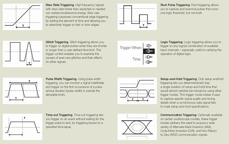
You can trigger on pulses defined by amplitude (such as runt pulses), qualified by time (pulse width, glitch, slew rate, setup-and-hold, and time-out), and delineated by logic state or pattern (logic triggering).
Other advanced trigger functions include:
Pattern Lock Triggering: Pattern lock triggering adds a new dimension to NRZ serial pattern triggering by enabling the oscilloscope to take synchronized acquisitions of a long serial test pattern with outstanding time base accuracy.
Pattern lock triggering can be used to remove random jitter from long serial data patterns. Effects of specific bit transitions can be investigated, and averaging can be used with mask testing.
Serial Pattern Triggering: Serial pattern triggering can be used to debug serial architectures. It provides a trigger on the serial pattern of an NRZ serial data stream with built-in clock recovery and correlates events across the physical and link layer.
The instrument can recover the clock signal, identify transitions, and allow you to set the desired encoded words for the serial pattern trigger to capture.
A & B Triggering: Some trigger systems offer multiple trigger types only on a single event (A event), with delayed trigger (B event) selection limited to edge type triggering and often do not provide a way to reset the trigger sequence if the B event doesn’t occur.
Modern oscilloscopes can provide the full suite of advanced trigger types on both A and B triggers, logic qualification to control when to look for these events, and reset triggering to begin the trigger sequence again after a specified time, state, or transition so that even events in the most complex signals can be captured.
Search & Mark Triggering: Hardware triggers watch for one event type at a time, but Search can scan for multiple event types simultaneously. For example, scan for setup or hold time violations on multiple channels. Individual marks can be placed by Search indicating events that meet search criteria.
Trigger Correction: Since the trigger and data acquisition systems share different paths there is some inherent time delay between the trigger position and the data acquired. This results in skew and trigger jitter.
With a trigger correction system the instrument adjusts the trigger position and compensates for the difference of delay there is between the trigger path and the data acquisition path. This eliminates virtually any trigger jitter at the trigger point. In this mode, the trigger point can be used as a measurement reference. Serial Triggering on Specific Standard Signals I2C, CAN, LIN, etc.):
Some oscilloscopes (compare Tektronix oscilloscopes) provide the ability to trigger on specific signal types for standard serial data signals such as CAN, LIN, I2C, SPI, and others. The decoding of these signal types is also available on many oscilloscopes.
Parallel Bus Triggering: Multiple parallel buses can be defined and displayed at one time to easily view decoded parallel bus data over time. By specifying which channels are the clock and data lines, you can create a parallel bus display on some oscilloscopes that automatically decodes bus content.
You can save countless hours by using parallel bus triggers to simplify capture and analysis. Optional trigger controls in some oscilloscopes are designed specifically to examine communications signals as well.
Figure 34 highlights a few of these common trigger types in more detail. To maximize your productivity, some oscilloscopes provide an intuitive user interface to allow rapid setup of trigger parameters with wide flexibility in the test setup.
Figure 34: Common trigger types.
Trigger Position
Horizontal trigger position control is only available on digital oscilloscopes. The trigger position control may be located in the horizontal control section of your oscilloscope. It actually represents the horizontal position of the trigger in the waveform record.
Varying the horizontal trigger position allows you to capture what a signal did before a trigger event, known as pre-trigger viewing. Thus, it determines the length of viewable signal both preceding and following a trigger point.
Digital oscilloscopes can provide pre-trigger viewing because they constantly process the input signal, whether or not a trigger has been received. A steady stream of data flows through the oscilloscope; the trigger merely tells the oscilloscope to save the present data in memory.
In contrast, analog oscilloscopes only display the signal—that is, write it on the CRT—after receiving the trigger. Thus, pre-trigger viewing is not available in analog oscilloscopes, with the exception of a small amount of pre-trigger provided by a delay line in the vertical system.
Pre-trigger viewing is a valuable troubleshooting aid. If a problem occurs intermittently, you can trigger on the problem, record the events that led up to it and, possibly, find the cause.
Trigger Level and Slope
The trigger level and slope controls provide the basic trigger point definition and determine how a waveform is displayed (Figure 35).
Figure 35: Positive and negative slope triggering.
The trigger circuit acts as a comparator. You select the slope and voltage level on one input of the comparator. When the trigger signal on the other comparator input matches your settings, the oscilloscope generates a trigger.
The slope control determines whether the trigger point is on the rising or the falling edge of a signal. A rising edge is a positive slope and a falling edge is a negative slope. The level control determines where on the edge the trigger point occurs.
Trigger Sources
The oscilloscope does not necessarily need to trigger on the signal being displayed. Several sources can trigger the sweep:
Any input channel
An external source other than the signal applied to an input channel
The power source signal
A signal internally defined by the oscilloscope, from one or more input channels
Most of the time, you can leave the oscilloscope set to trigger on the channel displayed. Some oscilloscopes provide a trigger output that delivers the trigger signal to another instrument.
The oscilloscope can use an alternate trigger source, whether or not it is displayed, so you should be careful not to unwittingly trigger on channel 1 while displaying channel 2, for example.
Trigger Modes
The trigger mode determines whether or not the oscilloscope draws a waveform based on a signal condition. Common trigger modes include normal and auto:
In normal mode the oscilloscope only sweeps if the input signal reaches the set trigger point. Otherwise, the screen is blank (on an analog oscilloscope) or frozen (on a digital oscilloscope) on the last acquired waveform. Normal mode can be disorienting since you may not see the signal at first if the level control is not adjusted correctly.
Auto mode causes the oscilloscope to sweep, even without a trigger. If no signal is present, a timer in the oscilloscope triggers the sweep. This ensures that the display will not disappear if the signal does not cause a trigger.
In practice, you will probably use both modes: normal mode because it lets you see just the signal of interest, even when triggers occur at a slow rate, and auto mode because it requires less adjustment. Many oscilloscopes also include special modes for single sweeps, triggering on video signals, or automatically setting the trigger level.
Trigger Coupling
Just as you can select either AC or DC coupling for the vertical system, you can choose the kind of coupling for the trigger signal.
Besides AC and DC coupling, your oscilloscope may also have high frequency rejection, low frequency rejection, and noise rejection trigger coupling. These special settings are useful for eliminating noise from the trigger signal to prevent false triggering.
Trigger Holdoff
Sometimes getting an oscilloscope to trigger on the correct part of a signal requires great skill. Many oscilloscopes have special features to make this task easier.
Trigger holdoff is an adjustable period of time after a valid trigger during which the oscilloscope cannot trigger. This feature is useful when you are triggering on complex waveform shapes, so that the oscilloscope only triggers on an eligible trigger point.
Figure 36 shows how using trigger holdoff helps create a usable display.
Figure 36: Positive and negative slope triggering.
Controls for Math and Measurement Operations
Your oscilloscope may also have operations that allow you to add waveforms together, creating a new waveform display. Analog oscilloscopes combine the signals while digital oscilloscopes create new waveforms mathematically. Subtracting waveforms is another math operation.
Subtraction with analog oscilloscopes is possible by using the channel invert function on one signal and then using the add operation. Digital oscilloscopes typically have a subtraction operation available. Figure 38 illustrates a third waveform created by combining two different signals.
Figure 38: Adding channels.
Using the power of their internal processors, digital oscilloscopes offer many advanced math operations: multiplication, division, integration, Fast Fourier Transform, and more.
This advanced signal processing capability can also perform functions such as the insertion of a filter block that can be used to de-embed the characteristics of the fixture on the device under test or implement a filter block with desired frequency response such as a low pass filter.
The processing block is flexible, not dedicated. It can perform as an arbitrary filter instead. For example, for simulation of pre-emphasis/de-emphasis schemes.
Digital Timing and State Acquisitions
Digital channels provided by a mixed signal oscilloscope enable acquisition capabilities similar to those found on logic analyzers. There are two major digital acquisition techniques:
With timing acquisition, the MSO samples the digital signal at uniformly spaced times determined by the MSO's sample rate. At each sample point, the MSO stores the signal's logic state and creates a timing diagram of the signal.
State acquisition defines special times that the digital signal's logic state is valid and stable. This is common in synchronous and clocked digital circuits. A clock signal defines the time when the signal state is valid. For example, the input signal stable time is around the rising clock edge for a D-Flip-Flop with rising edge clocking. The output signal stable time is around the falling clock edge for a D-Flip-Flop with rising edge clocking. Since the clock period of a synchronous circuit may not be fixed, the time between state acquisitions may not be uniform as it is in a timing acquisition.
A mixed signal oscilloscope's digital channels acquire signals similar to how a logic analyzer acquires signals in timing acquisition mode.
The MSO then decodes the timing acquisition into a clocked bus display and event table display, which is similar to the logic analyzer's state acquisition. This provides important information during debugging.
Other Controls
This chapter described the basic oscilloscope controls that a beginner needs to know about. Your oscilloscope may have other controls for various functions. Some of these may include:
Automatic parametric measurements
Measurement cursors
Keypads for mathematical operations or data entry
Printing capabilities
Interfaces for connecting your oscilloscope to a computer or directly to the Internet
Look over the other options available to you and read your oscilloscope’s manual to find out more about these other controls.
Setting Up and Using an Oscilloscope How-To Guide
Once you have an oscilloscope, there are basic things you need to do to set it up and begin using it. This chapter briefly describes these things. In particular, proper grounding is very important for safety reasons; not just for yourself but also for the integrated circuits (ICs) you are testing. Setting oscilloscope controls, calibrating the oscilloscope, connecting probes, and compensating the probes are also described, along with basic oscilloscope measurement techniques.
Proper Grounding
Proper grounding is an important step when you set up to take measurements or work on a circuit:
Properly grounding the oscilloscope protects you from a hazardous shock.
Properly grounding yourself protects your ICs from damage.
To ground the oscilloscope means to connect it to an electrically neutral reference point, such as earth ground. Ground your oscilloscope by plugging its three-pronged power cord into an outlet grounded to earth ground. Grounding the oscilloscope is necessary for safety. If a high voltage contacts the case of an ungrounded oscilloscope—any part of the case, including knobs that appear insulated—it can give you a shock. However, with a properly grounded oscilloscope, the current travels through the grounding path to earth ground rather than through you to earth ground.
Grounding is also necessary for taking accurate measurements with your oscilloscope. The oscilloscope needs to share the same ground as any circuits you are testing. Some oscilloscopes do not require separate connection to earth ground. These oscilloscopes have insulated cases and controls, which keeps any possible shock hazard away from the user.
If you are working with ICs, you also need to ground yourself. ICs have tiny conduction paths that can be damaged by static electricity that builds up on your body. You can ruin an expensive IC simply by walking across a carpet or taking off a sweater and then touching the leads of the IC. To solve this problem, wear a grounding strap, as shown in Figure 64. This strap safely sends static charges on your body to earth ground.
Figure 64: Typical wrist-type grounding strap.
Setting the Controls
After plugging in the oscilloscope, take a look at the front panel. As described at the beginning of Chapter 4—Oscilloscope Systems and Controls, the front panel is typically divided into three main sections labeled vertical, horizontal, and trigger. Your oscilloscope may have other sections, depending on the model and type. Notice the input connectors on your oscilloscope—this is where you attach the probes. Most oscilloscopes have at least two input channels and each channel can display a waveform on the screen. Multiple channels are useful for comparing waveforms. The front panel of a Mixed Signal Oscilloscope (MSO) willalso have digital inputs.
Some oscilloscopes have AUTOSET and/or DEFAULT buttons that can set up the controls in one step to accommodate a signal. If your oscilloscope does not have this capability, it is helpful to set the controls to standard positions before taking measurements.
Oscilloscope Instructions
Set the oscilloscope to display channel 1.
Set the vertical volts/division scale and position controls to mid–range positions.
Turn off the variable volts/division.
Turn off all magnification settings.
Set the channel 1 input coupling to DC.
Set the trigger mode to auto.
Set the trigger source to channel 1.
Turn trigger holdoff to minimum or off.
Set the horizontal time/division and position controls to mid-range positions.
Adjust channel 1 volts/division such that the signal occupies as much of the 10 vertical divisions as possible without clipping or signal distortion.
Calibrating the Instrument
In addition to proper oscilloscope setup, periodic instrument self-calibration is recommended for accurate measurements. Oscilloscope calibration is needed if the ambient temperature has changed more than 5° C (9° F) since the last self-calibration or once per week. In the oscilloscope menu, this can sometimes be initiated as Signal Path Compensation. Refer to the manual that accompanied your oscilloscope for more detailed instructions.
Connecting the Probes
Once you have properly grounded the oscilloscope and yourself, and you’ve set up the oscilloscope in standard positions, you are ready to connect a probe to your oscilloscope. A probe, if well-matched to the oscilloscope, enables you to access all of the power and performance in the oscilloscope and will ensure the integrity of the signal you are measuring. Measuring a signal requires two connections:
The probe tip connection
The ground connection
Probes often come with a clip attachment for grounding the probe to the circuit under test. In practice, you attach the grounding clip to a known ground in the circuit, such as the metal chassis of a product you are repairing, and touch the probe tip to a test point in the circuit.
Compensating the Probes
Passive attenuation voltage probes must be compensated to the oscilloscope. Before using a passive probe, you need to compensate it to balance its electrical properties to a particular oscilloscope. You should get into the habit of compensating the probe every time you set up your oscilloscope. A poorly adjusted probe can make your measurements less accurate. Figure 65 illustrates the effects on a 1 MHz test signal when using a probe that is not properly compensated.
Most oscilloscopes have a square wave reference signal available at a terminal on the front panel used to compensate the probe. General instructions to compensate the probe are as follows:
Attach the probe to a vertical channel.
Connect the probe tip to the probe compensation, i.e. square wave reference signal.
Attach the ground clip of the probe to ground.
View the square wave reference signal.
Make the proper adjustments on the probe so that the corners of the square wave are square.
Oscilloscope Measurement Techniques
The two most basic measurements you can make are:
Voltage measurements
Time measurements
Just about every other measurement is based on one of these two fundamental techniques.
This section discusses methods for taking measurements visually with the oscilloscope screen. This is a common technique with analog instruments, and also may be useful for “at-a-glance” interpretation of digital oscilloscope displays.
Note that most digital oscilloscopes include automated measurement tools that simplify and accelerate common analysis tasks, thus improving the reliability and confidence of your measurements. However, knowing how to make measurements manually as described here will help you understand and check the automatic measurements.
Voltage Measurements
Voltage is the amount of electric potential, expressed in volts, between two points in a circuit. Usually one of these points is ground (zero volts), but not always. Voltages can also be measured from peak-to-peak. That is, from the maximum point of a signal to its minimum point. You must be careful to specify which voltage you mean. The oscilloscope is primarily a voltage-measuring device. Once you have measured the voltage, other quantities are just a calculation away. For example, Ohm’s law states that voltage between two points in a circuit equals the current times the resistance. From any two of these quantities you can calculate the third using the formula shown below.
Voltage = Current x Resistance
Another handy formula is the power law, which states that the power of a DC signal equals the voltage times the current. Calculations are more complicated for AC signals, but the point here is that measuring the voltage is the first step toward calculating other quantities. Figure 66 shows the voltage of one peak (Vp) and the peak-to-peak voltage (Vp–p).
Figure 66: Voltage peak (Vp) and peak-to-peak voltage (Vp-p).
The most basic method of taking voltage measurements is to count the number of divisions a waveform spans on the oscilloscope’s vertical scale. Adjusting the signal to cover most of the display vertically makes for the best voltage measurements, as shown in Figure 67. The more display area you use, the more accurately you can read the measurement.
Figure 67: Measure voltage on the center vertical graticule line.
Many oscilloscopes have cursors that let you make waveform measurements automatically, without having to count graticule marks. A cursor is simply a line that you can move across the display. Two horizontal cursor lines can be moved up and down to bracket a waveform’s amplitude for voltage measurements, and two vertical lines move right and left for time measurements. A readout shows the voltage or time at their positions.
Time and Frequency Measurements
You can make time measurements using the horizontal scale of the oscilloscope. Time measurements include measuring the period and pulse width of pulses. Frequency is the reciprocal of the period, so once you know the period, the frequency is one divided by the period. Like voltage measurements, time measurements are more accurate when you adjust the portion of the signal to be measured to cover a large area of the display, as illustrated in Figure 68.
<
Figure 68: Measure time on the center horizontal graticule line.
Pulse Width and Rise Time Measurements
In many applications, the details of a pulse’s shape are important. Pulses can become distorted and cause a digital circuit to malfunction, and the timing of pulses in a pulse train is often significant.
Standard pulse measurements are pulse rise time and pulse width. Rise time is the amount of time a pulse takes to go from a low to high voltage. By convention, the rise time is measured from 10% to 90% of the full voltage of the pulse. This eliminates any irregularities at the pulse’s transition corners.
Pulse width is the amount of time the pulse takes to go from low to high and back to low again. By convention, the pulse width is measured at 50% of full voltage. Figure 69 illustrates these measurement points.
Figure 69: Rise time and pulse width measurement points.
Pulse measurements often require fine-tuning the triggering. To become an expert at capturing pulses, you should learn how to use trigger hold-off and how to set the digital oscilloscope to capture pre-trigger data, as described in Chapter 4—Oscilloscope Systems and Controls.. Horizontal magnification is another useful feature for measuring pulses, since it allows you to see fine details of a fast pulse.
Whether positive or negative, your feedback helps us continually improve the
Tek.com experience. Let us know if you're having trouble or if we're doing an outstanding job.
Whether positive or negative, your feedback helps us continually improve the
Tek.com experience. Let us know if you're having trouble or if we're doing an outstanding job.
Series 2600B System SourceMeter Instrument Reference Manual
This manual includes advanced operation topics and maintenance information. Programmers looking for a command
reference and users looking for an in-depth description of the way the instrument works (including
troubleshooting and optimization) should refer to this manual.
ATTENTION: please read the following terms and conditions carefully before downloading any documents from
this website. By downloading manuals from Tektronix' website, you agree to the following terms and
conditions:
Manuals for Products That Are Currently Supported:
Tektronix hereby grants permission and license to owners of Tektronix instruments to download and reproduce
the manuals on this website for their own internal or personal use. Manuals for currently supported products
may not be reproduced for distribution to others unless specifically authorized in writing by Tektronix,
Inc.
A Tektronix manual may have been revised to reflect changes made to the product during its manufacturing
life. Thus, different versions of a manual may exist for any given product. Care should be taken to ensure
that one obtains the proper manual version for a specific product serial number.
Manuals for Products That Are No Longer Supported:
Tektronix cannot provide manuals for measurement products that are no longer eligible for long term
support. Tektronix hereby grants permission and license for others to reproduce and distribute copies of any
Tektronix measurement product manual, including user manuals, operator's manuals, service manuals, and the
like, that (a) have a Tektronix Part Number and (b) are for a measurement product that is no longer
supported by Tektronix.
A Tektronix manual may be revised to reflect changes made to the product during its manufacturing life.
Thus, different versions of a manual may exist for any given product. Care should be taken to ensure that
one obtains the proper manual version for a specific product serial number.
This permission and license does not apply to any manual or other publication that is still available from
Tektronix, or to any manual or other publication for a video production product or a color printer product.
Disclaimer:
Tektronix does not warrant the accuracy or completeness of the information, text, graphics, schematics,
parts lists, or other material contained within any measurement product manual or other publication that is
not supplied by Tektronix or that is produced or distributed in accordance with the permission and license
set forth above.
Tektronix may make changes to the content of this website or to its products at any time without notice.
Limitation of Liability:
TEKTRONIX SHALL NOT BE LIABLE FOR ANY DAMAGES WHATSOEVER (INCLUDING, WITHOUT LIMITATION, ANY CONSEQUENTIAL
OR INCIDENTAL DAMAGES, DAMAGES FOR LOSS OF PROFITS, BUSINESS INTERRUPTION, OR FOR INFRINGEMENT OF
INTELLECTUAL PROPERTY) ARISING OUT OF THE USE OF ANY MEASUREMENT PRODUCT MANUAL OR OTHER PUBLICATION
PRODUCED OR DISTRIBUTED IN ACCORDANCE WITH THE PERMISSION AND LICENSE SET FORTH ABOVE.
Read Online
Series 2600B System SourceMeter Instrument Reference Manual
The following safety precautions should be observed before using this product and any associated instrumentation. Although some instruments and accessories would normally be used with nonhazardous voltages, there are situations where hazardous conditions may be present.
This product is intended for use by personnel who recognize shock hazards and are familiar with the safety precautions required to avoid possible injury. Read and follow all installation, operation, and maintenance information carefully before using the product. Refer to the user documentation for complete product specifications.
If the product is used in a manner not specified, the protection provided by the
product warranty may be impaired.
The types of product users are:
Responsible body is the individual or group
responsible for the use and maintenance of equipment, for ensuring that the equipment is operated within
its specifications and operating limits, and for ensuring that operators are adequately trained.
Operators use the product for its intended
function. They must be trained in electrical safety procedures and proper use of the instrument. They must
be protected from electric shock and contact with hazardous live circuits.
Maintenance personnel perform routine
procedures on the product to keep it operating properly, for example, setting the line voltage or
replacing consumable materials. Maintenance procedures are described in the user documentation. The
procedures explicitly state if the operator may perform them. Otherwise, they should be performed only by
service personnel.
Service personnel are trained to work on
live circuits, perform safe installations, and repair products. Only properly trained service personnel
may perform installation and service procedures.
Keithley products are designed for use with electrical signals that are
measurement, control, and data I/O connections, with low transient overvoltages, and must not be directly
connected to mains voltage or to voltage sources with high transient overvoltages. Measurement Category II
(as referenced in IEC 60664) connections require protection for high transient overvoltages often
associated with local AC mains connections. Certain Keithley measuring instruments may be connected to
mains. These instruments will be marked as category II or higher.
Unless explicitly allowed in the specifications, operating manual, and
instrument labels, do not connect any instrument to mains.
Exercise extreme caution when a shock hazard is present. Lethal voltage may be
present on cable connector jacks or test fixtures. The American National Standards Institute (ANSI) states
that a shock hazard exists when voltage levels greater than 30 V RMS, 42.4 V peak, or
60 VDC are present. A good safety practice is to expect that hazardous voltage is present in any
unknown circuit before measuring.
Operators of this product must be protected from electric shock at all times.
The responsible body must ensure that operators are prevented access and/or insulated from every
connection point. In some cases, connections must be exposed to potential human contact. Product operators
in these circumstances must be trained to protect themselves from the risk of electric shock. If the
circuit is capable of operating at or above 1000 V, no conductive part of the circuit may be exposed.
Do not connect switching cards directly to unlimited power circuits. They are
intended to be used with impedance-limited sources. NEVER connect switching cards directly to AC mains.
When connecting sources to switching cards, install protective devices to limit fault current and voltage
to the card.
Before operating an instrument, ensure that the line cord is connected to a
properly-grounded power receptacle. Inspect the connecting cables, test leads, and jumpers for possible
wear, cracks, or breaks before each use.
When installing equipment where access to the main power cord is restricted,
such as rack mounting, a separate main input power disconnect device must be provided in close proximity
to the equipment and within easy reach of the operator.
For maximum safety, do not touch the product, test cables, or any other
instruments while power is applied to the circuit under test. ALWAYS remove power from the entire test
system and discharge any capacitors before connecting or disconnecting cables or jumpers, installing or
removing switching cards, or making internal changes, such as installing or removing jumpers.
Do not touch any object that could provide a current path to the common side of
the circuit under test or power line (earth) ground. Always make measurements with dry hands while
standing on a dry, insulated surface capable of withstanding the voltage being measured.
For safety, instruments and accessories must be used in accordance with the
operating instructions. If the instruments or accessories are used in a manner not specified in the
operating instructions, the protection provided by the equipment may be impaired.
Do not exceed the maximum signal levels of the instruments and accessories.
Maximum signal levels are defined in the specifications and operating information and shown on the
instrument panels, test fixture panels, and switching cards.
When fuses are used in a product, replace with the same type and rating for
continued protection against fire hazard.
Chassis connections must only be used as shield connections for measuring
circuits, NOT as protective earth (safety ground) connections.
If you are using a test fixture, keep the lid closed while power is applied to
the device under test. Safe operation requires the use of a lid interlock.
If a screw is present, connect it to protective earth (safety ground)
using the wire recommended in the user documentation.
The symbol on an instrument means caution, risk of hazard.
The user must refer to the operating instructions located in the user documentation in all cases where the
symbol is marked on the instrument.
The symbol on an instrument means warning, risk
of electric shock. Use standard safety precautions to avoid personal contact with these voltages.
The symbol on an instrument shows that the surface may be
hot. Avoid personal contact to prevent burns.
The symbol indicates a connection terminal to
the equipment frame.
If this symbol is on a product, it indicates that mercury is present in
the display lamp. Please note that the lamp must be properly disposed of according to federal, state, and
local laws.
The WARNING heading in the user
documentation explains hazards that might result in personal injury or death. Always read the associated
information very carefully before performing the indicated procedure.
The CAUTION heading in the user
documentation explains hazards that could damage the instrument. Such damage may invalidate the warranty.
The CAUTION heading with the symbol in the user documentation explains hazards that
could result in moderate or minor injury or damage the instrument. Always read the associated information
very carefully before performing the indicated procedure. Damage to the instrument may invalidate the
warranty.
Instrumentation and accessories shall not be connected to humans.
Before performing any maintenance, disconnect the line cord and all test cables.
To maintain protection from electric shock and fire, replacement components in
mains circuits — including the power transformer, test leads, and input jacks — must be
purchased from Keithley. Standard fuses with applicable national safety approvals may be used if the
rating and type are the same. The detachable mains power cord provided with the instrument may only be
replaced with a similarly rated power cord. Other components that are not safety-related may be purchased
from other suppliers as long as they are equivalent to the original component (note that selected parts
should be purchased only through Keithley to maintain accuracy and functionality of the product). If you
are unsure about the applicability of a replacement component, call a Keithley office for information.
Unless otherwise noted in product-specific literature, Keithley instruments are
designed to operate indoors only, in the following environment: Altitude at or below 2,000 m (6,562 ft);
temperature 0 °C to 50 °C (32 °F to 122 °F); and pollution degree 1 or 2.
To clean an instrument, use a cloth dampened with deionized water or mild,
water-based cleaner. Clean the exterior of the instrument only. Do not apply cleaner directly to the
instrument or allow liquids to enter or spill on the instrument. Products that consist of a circuit board
with no case or chassis (e.g., a data acquisition board for installation into a computer) should never
require cleaning if handled according to instructions. If the board becomes contaminated and operation is
affected, the board should be returned to the factory for proper cleaning/servicing.
Safety precaution revision as of June 2018.
Introduction
Welcome
Thank you for choosing a Keithley Instruments product. The 2600B System
SourceMeter® instrument provides manufacturers of electronic
components and semiconductor devices with an instrument that combines source and measurement
capabilities in a single instrument called a source‑measure unit (also called a SMU). This
combination simplifies test processes by eliminating synchronization and connection issues associated
with multiple instrument solutions. A 2600B provides a scalable, high throughput, highly
cost‑effective solution for precision DC, pulse, and low frequency AC source-measure testing that
also maintains code compatibility throughout the Series 2600B instruments.
Extended warranty
Additional years of warranty coverage are available on many products. These valuable
contracts protect you from unbudgeted service expenses and provide additional years of protection at a
fraction of the price of a repair. Extended warranties are available on new and existing products.
Contact your local Tektronix office, sales partner, or distributor for details.
Contact information
If you have any questions after you review the information in this documentation,
please contact your local Tektronix office, sales partner, or distributor. You can also call the
Tektronix corporate headquarters (toll‑free inside the U.S. and Canada only) at
1‑800‑833‑9200. For worldwide contact numbers, visit tek.com/contact-tek.
Customer documentation
The documentation for the 2600B includes a Quick Start Guide, User's Manual, and
Reference Manual. A Quick Start Guide is provided as a hard copy with the instrument. You can also
access it from tek.com/keithley as an Adobe Acrobat .pdf file.
Quick Start Guide: Provides unpacking
instructions, describes basic connections, and reviews basic operation information. If you are new to
Keithley Instruments equipment, refer to the Quick Start Guide to take the steps needed to unpack, set
up, and verify operation.
User's Manual: Includes installation,
instrument description, operation, and maintenance information.
Reference Manual: Includes advanced
operation topics and maintenance information. Programmers looking for a command reference and users
looking for an in‑depth description of how the instrument works (including troubleshooting and
optimization) should refer to the Reference Manual.
KickStart Software: Enables quick test setup
and data visualization when using one or more instruments.
Test Script Builder (TSB): This software
provides an environment to develop a test program and the ability to load the test program onto the
instrument. Running a program loaded on the instrument eliminates the need to send individual commands
from the host computer to the instrument when running a test.
IVI-COM Driver: An IVI instrument driver you
can use to create your own test applications in C/C++, VB.NET, or C# programming languages. It can
also be called from other languages that support calling a DLL or ActiveX (COM) object. Refer to IVI Foundation for
additional information.
LabVIEW™ Software drivers: Drivers to
communicate with NITM LabVIEWTM Software.
Keithley I/O layer: Manages the
communications between Keithley instrument drivers and software applications and the instrument
itself. The I/O Layer handles differences in communications required to support GPIB, serial,
ethernet, and other communications buses so that drivers and software applications do not need to
handle the differences themselves.
To identify IP addresses of instruments that are connected to the local area network
(LAN) and support the VXI‑11 discovery protocol, you can also use LXI Discovery Tool, available
from the Resources page of the
LXI
Consortium website.
Capabilities and features
2600B System SourceMeter® instruments have the
following features:
4.5, 5.5, or 6.5 digit display resolution
Resistance and power measurement functions
Four-quadrant sink or source operation
Contact check function (not available on the 2604B, 2614B, and 2634B)
High‑capacitance mode for load impedance up to 50 µF (microfarads)
Linear, logarithmic, and custom sweeping and pulsing
Filtering to reduce reading noise
A trigger model that supports extensive triggering and synchronization schemes at
hardware speeds
Internal memory that stores five user setup options
Dedicated reading buffers that can each store and recall over 140,000
measurements; additional dynamic reading buffers can be created
USB flash drive access for saving data buffers, test scripts, and user setups
Digital I/O port that allows the 2600B to control other devices (digital I/O
lines not available on the Models 2604B, 2614B, and 2634B)
Compatible with Keithley IVy, a wireless I‑V characterization tool
LXI® version 1.4 Core 2011 compliant
Embedded TSP scripting engine that is accessible from any host interface;
responds to high‑speed test scripts comprised of instrument control commands
TSP-LinkTM expansion bus that allows TSP-enabled
instruments to trigger and communicate with each other; advanced Test Script Processor (TSPTM) scripting engine features enable parallel script execution across the
TSP‑Link network (not available on the 2604B, 2614B, and 2634B)
Supports IEEE-488 (GPIB), RS-232, Universal Serial Bus (USB), and ethernet local
area network (LAN) connections
Model-specific capabilities
Additional source and measure features:
Model 2601B, 2602B, and 2604B System SourceMeter® instruments:
Source ±DC voltage from 5 µV to 40.4 V
Source ±DC current from 100 pA to 3.03 A
Source ±pulse current up to 10 A
Measure ±pulse current up to 10 A
Measure ±DC voltage from 100 nV to 40.8 V
Measure ±DC current from 100 fA to 3.06 A
Model 2611B, 2612B, and 2614B System SourceMeter® instruments:
Source ±DC voltage from 5 µV to 202 V
Source ±DC current from 2 pA to 1.515 A
Source ±pulse current up to 10 A
Measure ±pulse current up to 10 A
Measure ±DC voltage from 100 nV to 204 V
Measure ±DC current from 100 fA to 1.53 A
Model 2634B, 2635B, and 2636B System SourceMeter® instruments:
Source ±DC voltage from 5 µV to 202 V
Source ±DC current from 1 fA to 1.515 A
Source ±pulse current up to 10 A
Measure ±pulse current up to 10 A
Measure ±DC voltage from 100 nV to 204 V
2635B and 2636B: Measure ±DC current from 100 aA to 1.53 A
2634B: Measure ±DC current from 1 fA to 1.53 A
Display the serial number
The instrument serial number is on a label on the rear panel of the instrument. You
can also access the serial number from the front panel using the front-panel keys and menus.
To display the serial number on the front panel:
If the 2600B is in remote operation, press the EXIT
(LOCAL) keyonce to place the instrument in local
operation.
Press the MENU key.
Use the navigation wheel to scroll to the SYSTEM-INFO menu item.
Press the ENTER key. The SYSTEM INFORMATION
menu is displayed.
Scroll to the SERIAL# menu item.
Press the ENTER key. The 2600B serial number
is displayed.
Sourcing and measuring
Basic operation
WARNING For the
Models 2611B, 2612B, 2614B, 2634B, 2635B, and 2636B, hazardous voltages may be present on all output and
guard terminals. To prevent electrical shock that could cause injury or death, never make or break
connections to the 2600B while the instrument is powered on. Turn off the equipment from the front panel
or disconnect the main power cord from the rear of the 2600B before handling cables. Putting the
equipment into standby does not guarantee that the outputs are powered off if a hardware or software
fault occurs.
Source-measure capabilities
From the front panel, you can configure the instrument to perform the following
source-measure operations:
Source voltage: Measure and display current,
voltage, resistance, or power
Source current: Measure and display voltage,
current, resistance, or power
Measure resistance: Display resistance
calculated from voltage and current components of measurement (can optionally specify source voltage
or source current value)
Measure power: Display power calculated from
voltage and current components of measurement (can optionally specify source voltage or source current
value)
Measure only (V or I): Display voltage or
current measurement
Voltage and current
The following table lists the source and measure limits for the voltage and current
functions. The full range of operation is explained in Operating boundaries.
Circuit configurations
The fundamental source-measure configurations for the 2600B are shown in the following
figures. When sourcing voltage, you can measure current or voltage, as shown in the following figure.
A
Current meter
+
-
Voltage source
V
Voltage meter
When sourcing current, you can measure voltage or current, as shown in the following
figure.
A
Current meter
?
Current source
V
Voltage meter
See the following topics for detailed information.
Source V
When configured to source voltage (V-source) as shown in the figure below, the 2600B
functions as a low-impedance voltage source with current limit capability and can measure current
(I-meter) or voltage (V-meter).
Sense circuitry is used to monitor the output voltage continuously and make
adjustments to the V‑source as needed. The V-meter senses the voltage at the HI / LO terminals
(2-wire local sense) or at the device under test (DUT) (4-wire remote sense using the sense terminals)
and compares it to the programmed voltage level. If the sensed level and the programmed value are not
the same, the V‑source is adjusted accordingly. Remote sense eliminates the effect of voltage
drops in the test leads, ensuring that the exact programmed voltage appears at the DUT. With 4-wire
sensing enabled, both remote sense leads must be connected or incorrect operation occurs. For the
2601B, 2602B, 2611B, 2612B, 2635B, and 2636B, use contact check to verify that the sense leads are
connected (see Contact check
measurements).
Source I
When the instrument is configured to source current (I-source), as shown in the
figure below, the instrument functions as a high-impedance current source with voltage limit
capability and can measure current (I-meter) or voltage (V-meter).
For 2-wire local sensing, voltage is measured at the HI / LO terminals of the instrument. For 4-wire remote sensing, voltage is measured directly at the device‑under‑test (DUT) using the sense terminals. This eliminates any voltage drops that may be in the test leads or connections between the instrument and the DUT.
The current source does not require or use the sense leads to enhance current source accuracy. However, if the instrument is in 4-wire remote sense mode, the instrument may reach limit levels if the sense leads are disconnected. With 4-wire remote sensing selected, the sense leads must be connected or incorrect operation results.
Source I measure I, source V measure V
The System SourceMeter® instrument can measure
the same function that it is sourcing. For example, when sourcing a voltage, you can measure voltage.
Conversely, if you are sourcing current, you can measure the output current. For these operations, the
measure range is the same as the source range.
This feature is valuable when operating with the source in compliance. When in
compliance, the programmed source value is not reached, so measuring the source lets you measure the
actual output level.
Measure only (voltage or current)
The figures below show the configurations for using the instrument exclusively as a
voltmeter or ammeter.
As shown in the following figure, to configure the instrument to measure voltage
only, set it to source 0 A and measure voltage.
Set the voltage limit to a level that is higher than the measured voltage. If the voltage
limit is set to a level that is lower than the measured voltage, excessive current flows into the
instrument. This current could damage the instrument. Also, when connecting an external energy source
to the instrument when it is configured as a current source, set the output off state to the
high-impedance mode. See Output-off states for more
information on the output-off states. See “Limits” in the Model 2600B User's Manual for details on compliance limits.
In the following figure, the instrument uses a 2-wire local sensing configuration
and is set to measure current only by setting it to source 0 V and measure current. Note that to
obtain positive (+) readings, conventional current must flow from HI to LO.
Contact check
The Models 2604B, 2614B, and 2634B do not perform contact check measurements.
When a contact check measurement is made, two small current sources switch between
the HI and SENSE HI terminals and the LO and SENSE LO terminals. By controlling the switches
illustrated in the following figure, the current from these sources flows through the test leads and
through the contact resistance, as shown. To accurately measure the resulting contact resistance, the
differential amplifier outputs are measured once with the current sources connected, and again with
the current sources disconnected. This allows for compensation of various offset voltages that can
occur.
The ADC of the 2600B uses a ratiometric analog to digital (A/D) conversion
technique. To ensure reading accuracy, the instrument must periodically obtain fresh measurements of
its internal ground and voltage reference. Separate reference and zero measurements are used for each
aperture.
As summarized in the table below, there are different settings for autozero. By
default, the instrument is set to AUTO, which automatically checks these reference measurements
whenever a signal measurement is made. If the reference measurements are out of date when a signal
measurement is made, the instrument automatically makes two more A/D conversions, one for the
reference and one for the zero, before returning the result. Thus, occasionally, a measurement takes
longer than normal.
This extra time can cause problems in sweeps and other test sequences in which
measurement timing is critical. To avoid the extra time for the reference measurements in these
situations, you can select OFF. This setting disables the automatic reference measurements. Note that
with automatic reference measurements disabled, the instrument may gradually drift out of
specification.
To minimize the drift, make a reference and zero measurement immediately before a
critical test sequence. You can use the ONCE setting to force a refresh of the reference and zero
measurements used for the current aperture setting.
Autozero settings
Autozero setting
Description
OFF
Turns automatic reference measurements off.
ONCE
After immediately making one reference and one zero measurement, turns
automatic reference measurements off.
AUTO
Automatically makes new acquisitions when the 2600B determines reference
and zero values are out-of-date.
Setting autozero from the front panel
To change autozero from the front panel:
Press the CONFIG key.
Press the MEAS key.
Turn the navigation wheel to select AUTO-ZERO, and then press the ENTER key or the navigation wheel.
Turn the navigation wheel to select the mode (OFF, ONCE, or AUTO), and then press the ENTER
key or the navigation wheel.
Press the EXIT (LOCAL) key to return to
the previous display.
Setting autozero from a remote interface
To set autozero from a remote interface:
Use the autozero command with the appropriate option shown in the following table to
set autozero through a remote interface (see smuX.measure.autozero). For example, send the following
command to activate channel A automatic reference measurements:
smua.measure.autozero = smua.AUTOZERO_AUTO
Autozero command and options
Command*
Description
smuX.measure.autozero = smuX.AUTOZERO_OFF
Disable autozero. Old NPLC cache values are used when autozero is
disabled (see NPLC
caching).
smuX.measure.autozero = smuX.AUTOZERO_ONCE
After immediately making one reference and one zero measurement, turns
automatic reference measurements off.
smuX.measure.autozero = smuX.AUTOZERO_AUTO
Automatically makes new reference and zero measurements when the 2600B
determines values are out-of-date.
* smuX can be smua for channel A or
smub for channel B
NPLC caching
NPLC caching speeds up operation by caching A/D reference and zero values for up to
the ten most recent measurement aperture settings. Whenever the integration rate is changed using the
SPEED key, or a user setup is recalled, the NPLC cache is checked. If the integration rate is already
stored in the cache, the stored reference and zero values are recalled and used. If the integration
rate is not already stored in the cache, a reference and zero value is acquired and stored in the
cache when the next measurement is made. If there are already ten NPLC values stored, the oldest one
is overwritten by the newest one. When autozero is off, NPLC values stored in the cache are used,
regardless of age.
Remote source-measure commands
Basic source-measurement procedures can also be performed through a remote interface.
To do this, send the appropriate commands. The following table summarizes basic source-measure commands.
See Introduction to TSP operation
for more information on using these commands.
Basic source-measure commands
Command*
Description
smuX.measure.autorangei = smuX.AUTORANGE_ON
Enable current measure autorange.
smuX.measure.autorangev = smuX.AUTORANGE_ON
Enable voltage measure autorange.
smuX.measure.autorangei = smuX.AUTORANGE_OFF
Disable current measure autorange.
smuX.measure.autorangev = smuX.AUTORANGE_OFF
Disable voltage measure autorange.
smuX.measure.rangei = rangeval
Set current measure range.
smuX.measure.rangev = rangeval
Set voltage measure range.
reading = smuX.measure.i()
Request a current reading.
reading = smuX.measure.v()
Request a voltage reading.
iReading, vReading = smuX.measure.iv()
Request a current and voltage reading.
reading = smuX.measure.r()
Request a resistance reading.
reading = smuX.measure.p()
Request a power reading.
smuX.source.autorangei = smuX.AUTORANGE_ON
Enable current source autorange.
smuX.source.autorangev = smuX.AUTORANGE_ON
Enable voltage source autorange.
smuX.source.autorangei = smuX.AUTORANGE_OFF
Disable current source autorange.
smuX.source.autorangev = smuX.AUTORANGE_OFF
Disable voltage source autorange.
smuX.source.func = smuX.OUTPUT_DCVOLTS
Select voltage source function.
smuX.source.func = smuX.OUTPUT_DCAMPS
Select current source function.
smuX.source.leveli = sourceval
Set current source value.
smuX.source.levelv = sourceval
Set voltage source value.
smuX.source.limiti = level
Set current limit.
smuX.source.limitv = level
Set voltage limit.
smuX.source.limitp = level
Set power limit.
smuX.source.output = smuX.OUTPUT_ON
Turn on source output.
smuX.source.output = smuX.OUTPUT_OFF
Turn off source output.
smuX.source.rangei = rangeval
Set current source range.
smuX.source.rangev = rangeval
Set voltage source range.
smuX.sense
= smuX.SENSE_LOCAL
Select local sense (2-wire).
smuX.sense
= smuX.SENSE_REMOTE
Select remote sense (4-wire).
* smuX can be smua for channel A or
smub for channel B
Requesting readings
You can request readings by including the appropriate measurement command as the
argument for the print() command. The
following programming example illustrates how to request a channel A current reading:
print(smua.measure.i())
Source-measure programming example
The following SMU programming example illustrates the setup and command sequence of
a basic source‑measure procedure with the following parameters:
Source function and range: Voltage, autorange
Source output level: 5 V
Current compliance limit: 10 mA
Measure function and range: Current, 10 mA
-- Restore 2600B defaults.
smua.reset()
-- Select voltage source function.
smua.source.func = smua.OUTPUT_DCVOLTS
-- Set source range to autorange.
smua.source.autorangev = smua.AUTORANGE_ON
-- Set voltage source to 5 V.
smua.source.levelv = 5
-- Set current limit to 10 mA.
smua.source.limiti = 10e-3
-- Set current range to 10 mA.
smua.measure.rangei = 10e-3
-- Turn on output.
smua.source.output = smua.OUTPUT_ON
-- Print and place the current reading in the reading buffer.
print(smua.measure.i(smua.nvbuffer1))
-- Turn off output.
smua.source.output = smua.OUTPUT_OFF
Triggering in local mode
You do not need to change any trigger settings to use the basic source and measurement
procedures described in the following topics.
Press the MENU key, and then select SETUP > RECALL > INTERNAL > FACTORY to reset the factory
default conditions.
The following figure shows the general sequence for SMU measurement triggering. The
basic sequence is as follows:
When the output is turned on, the programmed source value is immediately applied
to the device under test (DUT).
Through the front panel only: If the immediate trigger source is selected, a
measurement is triggered immediately. However, if the manual trigger source is selected, the
front‑panel TRIG key must be pressed.
The instrument waits for the programmed delay period (if any).
The instrument makes one measurement.
If the number of measurements is less than the programmed trigger count, it
cycles to make another measurement (the measurement cycle is repeated indefinitely if the infinite
trigger count is selected).
For multiple measurements, the instrument waits for the programmed trigger
interval (if any) before making the next measurement.
Configuring trigger attributes in local mode
From the front panel, press the CONFIG key, and
then select TRIG. The following menu items are available:
TRIGGER-IN: Use these options to select the
trigger-in source:
IMMEDIATE: Triggering occurs
immediately and the instrument starts to make measurements when it is ready (for example, after
the source output is turned on).
MANUAL: The front‑panel TRIG key
must be pressed to trigger the instrument to make readings.
COUNT: Sets the trigger count (number of
measurements) as follows:
FINITE: The instrument goes through
measurement cycles for the programmed trigger count (1 to 99999).
INFINITE: The instrument goes through
measurement cycles indefinitely until halted.
INTERVAL: Sets the time interval between
measurements (0 s to 999.999 s) when the count is greater than 1.
DELAY: Sets the delay period between the
trigger and the start of measurement (0 s to 999.999 s).
Front-panel triggering example
This example uses the front panel to configure the trigger parameters to meet the
following requirements:
Manual triggering (TRIG key)
Infinite trigger count (cycle indefinitely through measurement cycles)
Interval (time between measurements): 1 s
Delay (time from trigger to measurement): 2 s
To configure the trigger parameters:
Press the CONFIG key, and then the TRIG key.
Select TRIGGER-IN, and then press the
ENTER key or the navigation wheel.
Select MANUAL, and then press the ENTER key or the navigation wheel.
Select COUNT, then select INFINITE, and then press the ENTER key or thenavigation
wheel.
Select INTERVAL, set the interval to
1 s, and then press the ENTER key or thenavigation wheel.
Choose DELAY, set the delay to 2 s,
and then press the ENTER key or thenavigation wheel.
Use the EXIT (LOCAL) key to return to the
normal display.
Press the OUTPUT ON/OFF control to turn
the output on.
Press the TRIG key. A 2 s delay
occurs before the first measurement. The instrument cycles through measurements indefinitely with a
1 s interval between measurements.
Press the OUTPUT ON/OFF control again to
stop making readings.
Configuring for measure-only tests using the MODE key
In addition to using the 2600B for conventional source-measure operations, you can
also use it like a meter to measure current, voltage, resistance, or power.
To configure the 2600B as a voltage meter, current meter, ohmmeter, or
wattmeter:
Press the MODE key.
Turn the navigation wheel to select the type of meter from the menu (I‑METER, V-METER, OHM-METER, or WATT-METER).
Press the ENTER key to complete the
configuration of the 2600B as the selected meter.
To manually configure the settings, refer to the following topics:
You can make voltmeter and ammeter measurements without using the MODE key, such as
when configuring measure-only tests over the remote interface.
To use the 2600B to measure voltage or current:
Select the source-measure functions:
Voltmeter: Press the SRC key to select the current source and press the MEAS key to select the voltage measurement function.
Ammeter: Press the SRC key to select the voltage source and press the MEAS key to select the current measurement function.
Set source and compliance levels. To edit the source level, use the procedure
provided in Step 1: Select and set the source level; to edit the compliance level, use the procedure
provided in Step 2: Set the compliance limit:
Select the lowest source range and set the source level to zero.
Set the compliance level to a value that is higher than the expected
measurement.
When using the 2600B as a voltmeter, the voltage compliance limit must be set higher than the
voltage that is being measured. Failure to do this could result in excessive current flow into the
2600B, incorrect measurements, and possible damage to the instrument.
Use the RANGE keys to select a fixed
measurement range that accommodates the expected reading. Use the lowest possible range for best
accuracy. You can also select autorange, which automatically sets the 2600B to the most sensitive
range.
Connect the voltage or current to be measured. Make sure to use 2-wire
connections from the 2600B to the device under test (DUT) (see “DUT test connections” in
the Series 2600B User's Manual).
Press the OUTPUT ON/OFF control to turn the
output on.
View the displayed reading (press the TRIG
key if necessary).
When finished, press the OUTPUT ON/OFF
control to turn the output off.
Ohms measurements
Resistance readings are calculated from the measured current and measured voltage as
follows:
R = V/I
Where:
R is the calculated resistance
V is the measured voltage
I is the measured current
Ohms ranging
The front‑panel ohms function does not use ranging. The instrument formats a
calculated resistance reading (V/I) to best fit the display. There may be leading zeros if the ohms
reading is less than 1 mO.
Basic ohms measurement procedure
When you use the MODE key to select ohms measurement, the 2600B is automatically
configured as a current source with a level of 1 mA. To change the source function, source value,
or compliance value (in other words, customize the standard ohmmeter configuration of the MODE key),
then use the following steps to make ohms measurements. The following procedure assumes that the 2600B
is already connected to the device under test (see “DUT test connections” in the Series 2600B User's Manual).
The following procedure requires dual-channel instruments (2602B, 2604B, 2612B,
2614B, 2634B, and 2636B) to be placed in single-channel display mode. For these models, press the
DISPLAY key to select single-channel display mode. See
“Display mode” in the Series 2600B User's
Manual.
To make an ohms measurement:
Press the SRC key to select the source
function.
Set the output source, as indicated by the units in the source field on the
display. The flashing digit (cursor) indicates which value is presently selected for editing.
Move the cursor to the digit to change, then press the navigation wheel to
enter the EDIT mode.
Use the RANGE keys to select a range that
accommodates the value you want to set. For best accuracy, use the lowest possible
source range.
Enter the source value.
Press the ENTER key or the navigation
wheel to complete editing
Press the LIMIT key to edit the voltage or
current limit. When programming a voltage limit, set the voltage limit above the maximum expected
voltage across the resistor under test. When programming a current limit, set the current limit at
or above the maximum expected current through the resistor under test.
Move the cursor to the digit to change, then press the navigation wheel to
enter the EDIT mode, as indicated by the EDIT indicator.
Enter the limit value, then press the ENTER key or the navigation wheel to complete editing.
Press the MEAS key to display voltage or
current.
Make sure that AUTO measurement range is on (press the AUTO key if needed).
Press the MEAS key as many times as needed
to display ohms.
Press the OUTPUT ON/OFF control to turn
the output on.
View the displayed reading (press the TRIG
key if necessary). When finished, press the OUTPUT ON/OFF
control to turn the output off.
Remote ohms command
Use the smuX.measure.r() function to get a
resistance reading.
The programming example below illustrates how to get a resistance reading from SMU
A:
The following programming example illustrates the setup and command sequence of a
typical ohms measurement procedure with the following parameters:
Source function: Current, 10 mA
range, 10 mA output
Voltage measure range: Autorange
Voltage compliance: 10 V
Sense mode: 4‑wire
-- Restore 2600B defaults.
smua.reset()
-- Select the current source function.
smua.source.func = smua.OUTPUT_DCAMPS
-- Set the source range to 10 mA.
smua.source.rangei = 10e-3
-- Set the current source to 10 mA.
smua.source.leveli = 10e-3
-- Set the voltage limit to 10 V.
smua.source.limitv = 10
-- Enable 4-wire ohms.
smua.sense = smua.SENSE_REMOTE
-- Set the voltage range to auto.
smua.measure.autorangev = smua.AUTORANGE_ON
-- Turn on output.
smua.source.output = smua.OUTPUT_ON
-- Retrieve a resistance reading.
print(smua.measure.r())
-- Turn off output.
smua.source.output = smua.OUTPUT_OFF
Ohms sensing
Ohms measurements can be made using either 2-wire or 4-wire sensing. See “DUT
test connections” in the Series 2600B User's
Manual for information on connections and sensing methods.
The 2-wire sensing method has the advantage of requiring only two test leads.
However, as shown in the following figure (2-wire resistance sensing), test lead resistance can
seriously affect the accuracy of 2-wire resistance measurements, particularly with lower resistance
values.
The 4-wire sensing method, as shown in the following figure (4-wire resistance
sensing), minimizes or eliminates the effects of lead resistance by measuring the voltage across the
resistor under test with a second set of test leads. Because of the high input impedance of the
voltmeter, the current through the sense leads is negligible, and the measured voltage is essentially
the same as the voltage across the resistor under test.
Power measurements
Power readings are calculated from the measured current and voltage as follows:
Where:
P is the calculated power
V is the measured voltage
I is the measured current
Basic power measurement procedure
If you need to customize the standard wattmeter configuration of the MODE key,
perform the following steps to make power measurements. The following procedure assumes that the 2600B
is already connected to the device under test (DUT) as explained in “DUT test connections”
in the Series 2600B User's Manual.
Hazardous voltages may be present on all output and guard terminals. To prevent electrical
shock that could cause injury or death, never make or break connections to the 2600B while the output
is on. Turn off the equipment from the front panel or disconnect the main power cord from the rear of
the 2600B before handling cables. Putting the equipment into an output‑off state does not
guarantee that the outputs are powered off if a hardware or software fault occurs.
To perform power measurements from the front panel:
If the instrument has two channels (2602B, 2604B, 2612B, 2614B, 2634B, and
2636B), press the DISPLAY key to place it in single-channel
display mode.
Set source function and value. Press the SRC key to select the voltage or current source function, as
required.
Set the output voltage or current to an appropriate value.
Move the cursor to the digit to change, then press the navigation wheel to
enter the EDIT mode.
Use the RANGE keys to select a range that
accommodates the value you want to set. For best accuracy, use the lowest possible
source range.
Enter the source value.
Press the ENTER key or the navigation
wheel to complete editing.
Press the LIMIT key and set the voltage or
current limit high enough for the expected voltage or current across the DUT to be measured.
Press the LIMIT key.
Move the cursor to the digit to change, then press the navigation wheel to
enter the EDIT mode, as indicated by the EDIT indicator.
Enter the limit value, then press the ENTER key or the navigation wheel to complete editing.
Press the MEAS key as many times as needed
to display power.
Press the OUTPUT ON/OFF control to turn
the output on.
View the displayed reading (press the TRIG
key if necessary).
When finished, press the OUTPUT ON/OFF
control again to turn the output off.
Power measurements using the remote interface
The following paragraphs summarize basic power measurement commands using the remote
interface and also give a programming example for a typical power measurement situation.
Remote power reading command
The programming example below illustrates how to get a power reading from SMU A:
The following programming example illustrates the setup and command sequence for a
typical power measurement procedure with the following parameters:
Source function: Voltage, source
autorange, 5 V output
Current measure function and range:
Current, autorange
Current compliance: 50 mA
-- Restore 2600B defaults.
smua.reset()
-- Select voltage source function.
smua.source.func = smua.OUTPUT_DCVOLTS
-- Enable source autoranging.
smua.source.autorangev = smua.AUTORANGE_ON
-- Set voltage source to 5 V.
smua.source.levelv = 5
-- Set current limit to 50 mA.
smua.source.limiti = 50e-3
-- Set current range to autorange.
smua.measure.autorangei = smua.AUTORANGE_ON
-- Turn on the output.
smua.source.output = smua.OUTPUT_ON
-- Retrieve a power reading.
print(smua.measure.p())
-- Turn off the output.
smua.source.output = smua.OUTPUT_OFF
Contact check measurements
NOTE The Models 2604B, 2614B, and 2634B do not perform contact check
measurements.
The contact check function prevents measurements that may be in error due to excessive
resistance in the force or sense leads when making remotely sensed (Kelvin) measurements. Potential
sources for this resistance include poor contact at the device under test (DUT), failing relay contacts
on a switch card, and wires that are too long or thin. To use contact check, the current limit must be
at least 1 mA (this allows enough current to flow when performing the test), and the
source‑measure unit (SMU) must not be in High‑Z output‑off mode.
The contact check function also detects an open circuit that may occur when a
four-point probe is misplaced or misaligned. This relationship is shown schematically in the figure
below, where RC is the resistance of the mechanical contact at the DUT, and
RS is the series resistance of relays and cables.
When the source is off, smuX.source.offmode is set to
smuX.OUTPUT_ZERO, and the effective current limit is less than 1 mA, contact
check operations result in error code 5066, source.offlimiti too low for contact check. In the zero off mode, smuX.source.offlimiti is ignored and the effective current limit depends on what
the channel is sourcing when it is turned off. If the channel is sourcing:
Voltage: The current limit is determined by smuX.source.limiti.
Current: The current limit is determined by the greater of smuX.source.leveli or 10 percent of smuX.source.rangei.
Contact check commands
The following table summarizes the contact check commands. For a more complete
description of these commands, refer to the “TSP command
reference” section of the Series 2600B
Reference Manual.
Basic contact check commands
Command
Description
flag = smuX.contact.check()
Determine if contact resistance is lower than threshold.
rhi, rlo = smuX.contact.r()
Measure the aggregate contact resistance.
smuX.contact.speed = speedSetting
Set speedSetting to one of the
following:
0 or smuX.CONTACT_FAST
1 or smuX.CONTACT_MEDIUM
2 or smuX.CONTACT_SLOW
smuX.contact.threshold = rvalue
Set resistance threshold for the contact check function.
Contact check programming example
The following programming example illustrates the setup and command sequence for a
typical contact check measurement. These commands set the contact check speed to fast and the
threshold to 100 O. Then, a contact check measurement against the threshold is made. If it fails,
a more accurate contact check measurement is made, and the test is aborted. If it does not fail, the
output is turned on, and the test continues.
-- Restore defaults.
smua.reset()
-- Set contact-check speed to fast.
smua.contact.speed = smua.CONTACT_FAST
-- Set the contact-check threshold to 100 ohms.
smua.contact.threshold = 100
-- Check contacts against threshold.
if not smua.contact.check() then
-- Set speed to slow.
smua.contact.speed = smua.CONTACT_SLOW
-- Get aggregate resistance readings.
rhi, rlo = smua.contact.r()
-- Return contact resistances to the host.
print(rhi, rlo)
-- Terminate execution.
exit()
end
-- Turn output on and continue.
smua.source.output = smua.OUTPUT_ON
Multiple SMU connections
Connections to LO on the 2600B are not necessarily at 0 V. Hazardous voltages could exist
between LO and chassis ground. Make sure that high-voltage precautions are taken throughout the test
system. Alternatively, limit hazardous levels by adding external protection to limit the voltage between
LO and chassis. Failure to make sure high-voltage precautions are used throughout the test system or a
failure to limit hazardous levels could result in severe personal injury or death from electric shock.
Carefully consider and configure the appropriate output-off state, source function, and
compliance limits before connecting the 2600B to a device that can deliver energy (for example, other
voltage sources, batteries, capacitors, solar cells, or other 2600B instruments). Configure recommended
instrument settings before making connections to the device. Failure to consider the output-off state,
source, and compliance limits may result in damage to the instrument or to the device under test (DUT).
The following figures show how to use the SMUs of two 2600B instruments to test a
3-terminal device, such as an N-channel JFET. A typical application is for the 2600B to source a range
of gate voltages, while another 2600B sources voltage to the drain of the device and measures current at
each gate voltage.
Combining SMU outputs
The following information provides important considerations that need to be observed
when combining source‑measure unit (SMU) outputs.
Use care when combining SMUs. Whenever SMUs are combined, make sure both SMUs have the
same model number.
For further information, visit tek.com/keithley for application notes
on combining SMU channels, including Application Note 3047, Methods to Achieve
Higher Currents from I-V Measurement Equipment.
Carefully consider and configure the appropriate output-off state, source function, and
compliance limits before connecting the 2600B to a device that can deliver energy (for example, other
voltage sources, batteries, capacitors, solar cells, or other 2600B instruments). Configure recommended
instrument settings before making connections to the device. Failure to consider the output-off state,
source, and compliance limits may result in damage to the instrument or to the device under test (DUT).
Pulse characteristics for the 2601B, 2602B, and 2604B
The following figure and table illustrate the pulse regions for each SMU. The
programmed current and voltage levels for both SMUs must fall within the same pulse region. Refer to
the 2600B specifications on tek.com/keithley for the latest
pulse width and duty cycle information. Measurements are given priority over source and display
operations, so make sure that the measurement time does not exceed the allowable pulse width and duty
cycle in a particular pulse region.
Pulse region specification
Region (quadrant diagram)
Region maximum
Maximum pulse width
Maximum duty cycle
1
1 A at 40 V
DC, no limit
100%
1
3 A at 6 V
DC, no limit
100%
2
1.5 A at 40 V
100 ms
25%
3
5 A at 35 V
4 ms
4%
4
10 A at 20 V
1.8 ms
1%
5
5 A at 6 V
10 ms
10%
Pulse characteristics for the 2611B, 2612B, 2614B, 2634B, 2635B, and
2636B
The following figure and table illustrate the pulse regions for each SMU. The
programmed current and voltage levels for both SMUs must fall within the same pulse region. Refer to
the 2600B specifications on tek.com/keithley for the latest
pulse width and duty cycle information. Measurements are given priority over source and display
operations, so make sure that the measurement time does not exceed the allowable pulse width and duty
cycle in a particular pulse region.
Pulse region specifications
Region (quadrant diagram)
Region maximum
Maximum pulse width
Maximum duty cycle
1
100 mA at 200 V
DC, no limit
100%
1
1.5 A at 20 V
DC, no limit
100%
2
1 A at 180 V
8.5 ms
1%
3
1 A at 200 V
2.2 ms
1%
4
10 A at 5 V
1 ms
2.2%
Guidelines for combining SMU outputs
When combining the outputs of two 2600B SMUs, restrict operation to pulse only or
limited duty cycle operations whenever possible. DC operation in Region 1 is possible
if necessary.
Do not place two voltage sources in parallel.
Do not place two current sources in series.
Carefully consider the appropriate output-off mode (smua.source.offmode) and output-off function (smua.source.offfunc) whenever changes are made to the source function. An
alternative is to always use the high impedance output-off mode (smua.source.offmode = smua.OUTPUT_HIGH_Z).
To obtain the cleanest pulse edges and sweep steps, the rise and fall times of the
individual SMUs must be similar. For comparable rise and fall times, the source range, source level,
and limit range of SMU 1 should match the source range, source level, and limit range of SMU 2.
Because you cannot set the source limit range directly, you must choose limit values that cause both
SMUs to operate on the same limit range.
Additional configuration guidelines are presented in the following topics.
Additional information, including examples of combining SMU instruments, is available in application
notes on tek.com/keithley.
Source current using two 2600B instruments in parallel
This example shows the recommended approach for setting the source and limit ranges
and levels when combining SMU current sources in parallel.
The values are based on the current and voltage levels available in Region 4 of a
2601B, 2602B, or 2604B SMU, as shown in the table in Combining SMU outputs. For information about
generating pulses with a 2600B, refer to Using timers to perform pulse mode sweeps.
This configuration allows the combined SMUs to supply more current than a single SMU
current source can provide. In this example, SMU 1 and SMU 2 each supply one-half of the
total current for the SMU combination.
In this configuration, it is best practice to use only one SMU to limit the voltage
output of the SMU combination. In this example, SMU 2 limits the voltage. A good approach for
making sure that both SMUs are set to the same source limit range, which is recommended, is to set
SMU 1 to the maximum voltage allowed in Region 4, then set the limit for SMU 2 ten percent
lower.
A 10% source limit margin is generally recommended, but this value can be adjusted to meet
the requirements of a specific application.
Configure two 2600B SMUs to get the maximum pulsed
current level possible in Region 4:
20 A with 18 V source limit
SMU 1 configuration (sources one-half of the total pulse
current):
Source function:
smua.source.func = smua.OUTPUT_DCAMPS
Source range:
smua.source.rangei = 10
Idle (bias) source level (source level at the base of pulse):
smua.source.leveli = 0
Idle (bias) source limit (source limit at base of pulse):
smua.source.limitv = 6
Pulse source level (source level at top of pulse):
smua.trigger.source.listi({10})
Pulse source limit. SMU 2 controls the source limit for the combined SMUs. Set the
voltage source limit of SMU 1 to the maximum voltage allowed in Region 4:
smua.trigger.source.limitv = 20
Output-off mode:
smua.source.offmode = smua.OUTPUT_NORMAL
Output-off function:
smua.source.offfunc = smua.OUTPUT_DCAMPS
Normal output-off voltage limit:
smua.source.offlimitv = 20
SMU 2 configuration (sources one-half of the total pulse
current):
Source function:
smua.source.func = smua.OUTPUT_DCAMPS
Source range:
smua.source.rangei = 10
Idle (bias) source level (source level at base of pulse):
smua.source.leveli = 0
Idle (bias) source limit (source limit at base of pulse). Set the SMU 2 idle source
limit ten percent lower than the SMU 1 idle source limit:
smua.source.limitv = 5.4
Pulse source level (source level at top of pulse):
smua.trigger.source.listi({10})
Pulse source limit. SMU 2 controls the source limit for the combined SMUs. Set the
voltage source limit of SMU 2 ten percent lower than the source limit of SMU 1:
smua.trigger.source.limitv = 18
Output-off mode:
smua.source.offmode = smua.OUTPUT_NORMAL
Output-off function:
smua.source.offfunc = smua.OUTPUT_DCVOLTS
Current limit for normal output-off mode (this is the maximum current that flows
between the two SMUs when the output is off):
smua.source.offlimiti = 1e-3 -- default
Voltage compliance must be ten percent lower than the voltage compliance of SMU 1.
This causes SMU 1 to control the maximum voltage across the DUT. Voltage compliance limit
(maximum):
smua.trigger.source.limitv = 18
Source voltage using two 2600B instruments in series
This example shows the recommended approach for setting the source and limit ranges
and levels when combining SMU voltage sources in series.
The following values are based on the current and voltage levels available in Region
4 of a 2601B, 2602B, or 2604B SMU, as shown in the table in Combining SMU outputs. For information about
generating pulses with a 2600B, refer to Using timers to perform pulse mode sweeps.
This configuration supplies more voltage than a single SMU voltage source can
provide. In this example, SMU 1 and SMU 2 each supply one-half of the total voltage for the SMU
combination. For the back-to-back series connection shown, the total voltage of the combined SMUs is
VSMU 2 - VSMU 1. To obtain a net
differential voltage that is twice VSMU 2, the polarity of SMU 1 is
set to the opposite of the polarity of SMU 2.
In this configuration, it is best practice to use only one SMU to limit the current
output of the SMU combination. In this example, SMU 2 limits the current. A good approach for
making sure that both SMUs are set to the same source limit range, which is recommended, is to set
SMU 1 to the maximum current allowed in Region 4, then set the limit for SMU 2 ten percent
lower.
A 10% source limit margin is generally recommended, but this value can be adjusted to meet
the requirements of a specific application.
Configure two 2600B SMUs to get the maximum pulsed
voltage level possible in Region 4:
40 V with 9 A source limit
SMU 1 configuration (sources one-half of the total pulse
voltage):
Source function:
smua.source.func = smua.OUTPUT_DCVOLTS
Source range:
smua.source.rangev = 20
Idle (bias) source level (source level at base of pulse):
smua.source.levelv = -1e-12
Source polarity changes incur a 100 µs settling delay. Because the number 0 is treated as a
positive value in the 2600B, negative-going pulses with a 0 V bias level require the source to change
polarity. To ensure the proper pulse timing of SMU 1 and SMU 2, it is best to eliminate the SMU 1
polarity changes and avoid the associated 100 µs time penalty. The easiest way to do this is set the
bias level to a negative value that is significantly less than the programming resolution of the
instrument, such as -1e-12. Functionally, this value is the same as zero, but it is mathematically
negative, which eliminates the polarity change.
Idle (bias) source limit (source limit at base of pulse):
smua.source.limiti = 1
Pulse source level (source level at top of pulse):
smua.trigger.source.listv({-20})
As explained in the note above, the polarity of SMU 1 is generally the opposite of
the voltage polarity across the device. To achieve a positive voltage across the device, program SMU 1
to a negative voltage level. For example, to output 40 V across the device, program SMU 1 to -20 V and
SMU 2 to +20 V. To achieve a negative voltage across the device, program SMU 1 to a positive voltage
level and SMU 2 to a negative voltage level.
Pulse source limit. SMU 2 controls the source limit for the combined SMUs. Set the
current source limit of SMU 1 to the maximum current allowed in Region 4:
smua.trigger.source.limiti = 10
Output-off mode:
smua.source.offmode = smua.OUTPUT_NORMAL
Output-off function:
smua.source.offfunc = smua.OUTPUT_DCVOLTS
Normal output-off current limit:
smua.source.offlimiti = 1e-3 --(default)
SMU 2 configuration (sources one-half of the total pulse
voltage):
Source function:
smua.source.func = smua.OUTPUT_DCVOLTS
Source range:
smua.source.rangev = 20
Idle (bias) source level (source level at base of pulse):
smua.source.levelv = 0
Idle (bias) source limit (source limit at base of pulse). This is similar to the
pulse source limit. Set the SMU 2 idle source limit ten percent lower than the SMU 1 limit:
smua.source.limiti = 0.9
Pulse source level (source level at top of pulse):
smua.trigger.source.listv({-20})
Pulse source limit. SMU 2 controls the source limit for the combined SMUs. Set the
current source limit of SMU 2 ten percent lower than the source limit of SMU 1:
smua.trigger.source.limiti = 9
Output-off mode:
smua.source.offmode = smua.OUTPUT_NORMAL
Output-off function:
smua.source.offfunc = smua.OUTPUT_DCVOLTS
Normal output-off current limit (0.9 mA, which is 10% less than the SMU 1
output-off limit):
smua.source.offlimiti = 0.9e-3
Source voltage with extended current using two 2600B instruments in
parallel
This example shows the recommended approach for setting the source and limit ranges
and levels when combining a SMU voltage source in parallel with a SMU current source.
The values are based on the current and voltage levels available in Region 4 of a
2601B, 2602B, or 2604B SMU, as shown in the table in Combining SMU outputs. For information about
generating pulses with a 2600B, refer to Using timers to perform pulse mode sweeps.
The purpose of this configuration is to supply more current than a single SMU
voltage source can provide. In this example, SMU 2 controls the voltage applied to a device-under-test
(DUT). At full power, SMU 1 supplies 47% of the current required by the load and SMU 2 supplies 53%.
SMU2 sinks excess current from SMU 1 when DUT current draw is less than the maximum current of
the SMU combination.
Proper operation of this configuration requires that SMU 1 does not limit the
voltage from SMU 2 and that SMU 2 does not limit the current from SMU 1. To accomplish
this:
Set the voltage source level of SMU 2 ten percent lower than voltage source
limit of SMU 1.
Set the current source level of SMU 1 ten percent lower than the current source
limit of SMU 2.
Set the voltage source limit of SMU 1 to the maximum voltage allowed in Region
4.
Set the current source limit of SMU 2 to the maximum current allowed in Region
4.
These settings ensure that both SMUs are set to the same source and limit ranges, as
recommended.
A 10% source limit margin is generally recommended, but this value can be adjusted to meet
the requirements of a specific application.
Configure two 2600B SMUs to obtain the maximum pulsed
voltage level possible in Region 4:
18 V with 19 A capacity
SMU 1 configuration (supplies additional current that
SMU 2 alone cannot provide):
Source function:
smua.source.func = smua.OUTPUT_DCAMPS
Source range:
smua.source.rangei = 10
Idle (bias) source level (source level at base of pulse):
smua.source.leveli = 0
Idle (bias) source limit (source limit at base of pulse):
smua.source.limitv = 6
Pulse source level (source level at top of pulse). Set the pulse source level ten
percent lower than the current source limit of SMU 2:
smua.trigger.source.listi({9})
Pulse source limit. SMU 1 voltage source limit must be greater than the maximum
voltage supplied by SMU 2. Set the voltage source limit of SMU 1 to the maximum voltage allowed in
Region 4:
smua.trigger.source.limitv = 20
Output-off mode:
smua.source.offmode = smua.OUTPUT_NORMAL
Output-off function:
smua.source.offfunc = smua.OUTPUT_DCAMPS
Normal output-off voltage limit (40 V maximum):
smua.source.offlimitv = 20
SMU 2 configuration (SMU 2 controls the voltage applied
to the device‑under‑test):
Source function:
smua.source.func = smua.OUTPUT_DCVOLTS
Source range:
smua.source.rangev = 20
Idle (bias) source level (source level at base of pulse):
smua.source.levelv = 0
Idle (bias) source limit (source limit at base of pulse):
smua.source.limiti = 1
Pulse source level (source level at top of pulse). Set the source level of SMU 2 ten
percent lower than the voltage source limit of SMU 1:
smua.trigger.source.listv({18})
Pulse source limit. The pulse current source limit of SMU 2 must be greater than the
maximum current supplied by SMU 1. Set the current source limit of SMU 2 to the maximum current level
allowed in Region 4:
smua.trigger.source.limiti = 10
Output-off mode:
smua.source.offmode = smua.OUTPUT_NORMAL
Output-off function:
smua.source.offfunc = smua.OUTPUT_DCVOLTS
Normal output-off current limit:
smua.source.offlimiti = 1e-3
Combining channels in series to output higher voltage
Channels in series can cause hazardous voltage (>30 VRMS, 42 VPEAK) to be present and
accessible at the 2600B output connector. A safety shield must be used whenever hazardous voltages
will be present in the test circuit. To prevent electrical shock that could cause injury or death,
never use the 2600B in a test circuit that may contain hazardous voltages without a properly installed
and configured safety shield.
When combining two 2600B SMU voltage sources in series, it is possible for the SMU
combination to output hazardous voltage levels even though the individual SMUs cannot.
The following figure illustrates a Model 2602B configured with the two channels
connected in series to output up to 80 V (40 V per channel).
Whenever hazardous voltage (>30 VRMS,
42 VPEAK) is output, a safety shield must completely surround the
DUT test circuit. When using a metal safety shield, it must be connected to a known protective earth
(safety ground) and chassis ground.
(1) 2602B Channel A: SMU maximum pulse voltage: +40 V (2) 2602B Channel B:
SMU maximum pulse voltage: -40 V (3) Series SMU maximum pulse voltage (as shown): 80 V
Combining channels in parallel to output higher current
Higher pulse current can be output by connecting two 2600B instrument channels in
parallel.
The figure below illustrates the connection scheme of two Model 2602B channels
connected in parallel. Two Model 2602B channels can output up to 20 A at 18 V (see Combining SMU outputs). The current delivered to the
device under test (DUT) is the sum of the currents output by SMU channels (IT). Combining the two 2600B instrument channels expands the power envelope.
I1 Single SMU maximum pulse current: 10 A I2 Single SMU maximum pulse current: 10 A IT
Paralleled SMU channels maximum pulse current (as shown): 20 A
Output-off modes
CAUTION Carefully consider and configure the appropriate output-off state,
source function, and compliance limits before connecting the 2600B to a device that can deliver energy
(for example, other voltage sources, batteries, capacitors, solar cells, or other 2600B instruments).
Configure recommended instrument settings before making connections to the device. Failure to consider
the output-off state, source, and compliance limits may result in damage to the instrument or to the
device under test (DUT).
Turning off the 2600B output may not completely isolate the instrument from the
external circuit. You can use the output‑off mode to place the 2600B in a noninteractive state
during idle periods. The available output‑off modes are normal, high‑impedance, and zero.
Normal output-off mode
The normal output‑off mode is the default output‑off mode setting. When
the source‑measure unit (SMU) is in the normal output‑off mode, you can select either the
current or the voltage output‑off function (see Output-off function). You can also specify
current and voltage output‑off limits (Output-off limits (compliance)).
When the output is turned off, the output goes to either 0 V or 0 A, depending on
the selected output‑off function. Voltage is the default output‑off function.
High-impedance output-off mode
For the high-impedance output-off mode (HI‑Z), the output relay opens when the
output is turned off. This disconnects external circuitry from the input and output of the
source‑measure unit (SMU). To prevent excessive wear on the output relay, do not use this
output-off mode for tests that turn the output off and on frequently.
Zero output-off mode
When the zero output‑off mode is selected, the programmed source remains on
the display, but internally, the voltage source is selected and is set to 0 V. Measurements are
made and displayed.
When the selected source is voltage, the current compliance setting remains the same
as the output‑on value and compliance detection remains active.
When the selected source is current, the current compliance setting is the
programmed current source value or 10 percent full-scale of the present current range, whichever
is greater.
You can use the 2600B as a current meter when it is in zero output‑off mode
because it outputs 0 V but measures current.
To configure the output-off mode from the front panel:
Press the CONFIG key.
Press the OUTPUT ON/OFF control.
Select OFF-STATE.
Select MODE.
Select the output-off mode: HI-Z
(high‑impedance), NORMAL, or ZERO.
Press the EXIT key to return to the normal
display.
To select the normal output-off mode over a remote interface:*
smua.source.offmode = smua.OUTPUT_NORMAL
To select the high-impedance output-off mode over a remote interface:*
smua.source.offmode = smua.OUTPUT_HIGH_Z
To select the zero output-off mode over a remote interface:*
smua.source.offmode = smua.OUTPUT_ZERO
* smuX can be
smua for channel A or smub for channel B
Output-off function
This setting is used only when the output is turned off and the 2600B is set to the
normal output‑off mode (smuX.source.offmode = smuX.OUTPUT_NORMAL).
You can set the output-off function to CURRENT or VOLTAGE through the CONFIG menu on
the front panel, or by using the smuX.source.offfunc attribute from a
remote interface. VOLTAGE is the default output‑off function.
When the output is turned off and the selected output‑off function is VOLTAGE
(smuX.source.offfunc = smuX.OUTPUT_DCVOLTS):
The source‑measure unit (SMU) sources 0 V.
The current limit is set by the smuX.source.offlimiti attribute
(default 1 mA).
When the output is turned off and the selected output‑off function is CURRENT
(smuX.source.offfunc = smuX.OUTPUT_DCAMPS):
The SMU sources 0 A.
The voltage limit is set by the smuX.source.offlimitv attribute
(default 40 V).
When the output-off function is set to either voltage or current, the SMU may source
or sink a very small amount of power. In most cases, this source or sink power level is insignificant.
Selecting the output-off function
NOTE This setting is
used only when the output is turned off and the source‑measure unit (SMU) is in NORMAL
output‑off mode.
To configure the output-off function from the front panel:
Press the CONFIG key.
Press the OUTPUT ON/OFF control.
Select OFF-STATE and then select FUNCTION.
Select CURRENT or VOLTAGE.
Press the EXIT key to return to the normal
display.
To configure the output-off function remotely:
To set 0 V output with current limit set by the smuX.source.offlimiti attribute:*
smuX.source.offfunc
= smuX.OUTPUT_DCVOLTS
To set 0 A output with voltage limit set by the smuX.source.offlimitv attribute:*
smuX.source.offfunc
= smuX.OUTPUT_DCAMPS
* smuX can be
smua for channel A or smub for channel B
Output-off limits (compliance)
You can set output-off limits (compliance) for the current and voltage
output‑off functions using the CONFIG menu on the 2600B front panel, or by setting the smuX.source.offlimitY attribute from a
remote interface. The output‑off limits only apply when the output-off mode is normal.
Setting output-off limits
Setting the output‑off limit for CURRENT (smuX.source.offlimiti) specifies the current limit for the voltage source;
setting the output‑off limit for VOLTAGE (smuX.source.offlimitv) specifies the
voltage limit for the current source.
To configure the output-off limits from the front panel:
Press the CONFIG key.
Press the OUTPUT ON/OFF control.
Select OFF-STATE and then select LIMIT.
Select CURRENT or VOLTAGE.
Set the limit value and then press the ENTER key or the navigation wheel.
Press the EXIT key to return to the normal
display.
To set the current limit in NORMAL output‑off mode remotely:*
smuX.source.offlimiti = iValue
To set the voltage limit in NORMAL output‑off mode remotely:*
smuX.source.offlimitv = vValue
* smuX can be
smua for channel A or smub for channel B
Remote programming output-off states quick reference
The content of the following table is a quick reference of commands for programming
output-off states from a remote interface.
Output-off state programming quick reference
Command*
Description
smuX.source.offmode = smua.OUTPUT_NORMAL
Selects normal output‑off mode.
smuX.source.offmode = smua.OUTPUT_HIGH_Z
Selects high‑impedance output‑off mode.
smuX.source.offmode = smua.OUTPUT_ZERO
Selects zero output-off mode.
smuX.source.offfunc = smua.OUTPUT_DCVOLTS
Sets 0 V output with current limit specified by the smua.source.offlimiti attribute.
smuX.source.offfunc = smua.OUTPUT_DCAMPS
Sets 0 A output with voltage limit specified by the smua.source.offlimitv attribute.
smuX.source.offlimiti = iValue
Sets current limit in normal output‑off mode.
smuX.source.offlimitv = vValue
Sets voltage limit in normal output‑off mode.
* smuX can be smua for channel A or
smub for channel B
Range
The selected measurement range affects the accuracy of the measurements and the
maximum signal that can be measured. If the range is changed, the front‑panel display may contain
dashes instead of a reading (for example, --.---- mA). This indicates
that no measurement was made using the range that is presently selected. To update the displayed
reading, trigger a measurement (if in local control, press the TRIG key).
Available ranges
The following table lists the available source and measurement ranges for the 2600B.
2601B, 2602B, or 2604B
2611B, 2612B, or 2614B
2634B, 2635B, or 2636B
Voltage ranges
Current ranges
Voltage ranges
Current ranges
Voltage ranges
Current ranges
100 mV
100 nA
200 mV
100 nA
200 mV
100 pA2,3
1 V
1 µA
2 V
1 µA
2 V
1 nA
6 V
10 µA
20 V
10 µA
20 V
10 nA
40 V
100 µA
200 V
100 µA
200 V
100 nA
1 mA
1 mA
1 µA
10 mA
10 mA
10 µA
100 mA
100 mA
100 µA
1 A
1 A
1 mA
3 A
1.5 A
10 mA
10 A1
100 mA
1 A
1.5 A
1. The 10 A range is only available in pulse mode.
2. The 100 pA range is only for measurements.
3. The 100 pA measurement range is not available on the 2634B.
Maximum source values and readings
The full-scale output for each voltage and current source range is 101 percent of
the selected range, but the full-scale measurement is 102 percent of the range. For example,
±1.01 A is the full-scale source value for the 1 A range, and ±102 mA is the full-scale
reading for the 100 mA measurement range. Input levels that exceed the maximum levels cause the
overflow message to be displayed. The instrument autoranges at 100 percent of the range.
Measure autodelay
The measure delay is a specific delay that is applied before each measurement is
made. This delay is disabled by default (measurements are made immediately). You can change the
default delay by setting the smuX.measure.delay attribute either to a specific value
or to an autodelay setting (set smuX.measure.delay = smuX.DELAY_AUTO). If the measure delay is
set to the autodelay setting, a range-dependent delay is applied each time the instrument performs a
current measurement. This delay also happens for the measurement that is made after changing current
ranges during an autoranged measurement. The default measurement delay varies by model.
You can increase or decrease the autodelay by changing the delay factor (for
example, to reduce the delay across all ranges by half, set smuX.measure.delayfactor = 0.5). For
additional information, refer to smuX.measure.delayfactor.
Ranging limitations
If the source and measure functions are different (such as source V and measure I,
or source I and measure V), you can set source and measure ranges separately. If both the source
and the measure functions are the same, the measure range is locked to the source range. In addition,
there are other limitations.
2601B, 2602B, 2604B: With the 40 V
V‑Source range selected, the highest current measurement range is 1 A. With the 3 A
I‑Source range selected, the highest voltage measurement range is 6 V. Refer to Operating
boundaries for power derating information.
2611B, 2612B, 2614B, 2634B, 2635B, 2636B:
With the 200 V V-Source range selected, the highest current measurement range is
100 mA. With I-Source ranges above 100 mA selected, the highest voltage measurement range is
20 V. Refer to Operating boundaries for power derating information.
Manual ranging
Use the range keys, and , to select a fixed range:
To set the source range, press the SRC
key, and then use the RANGE keys to set the range.
To set the measure range, select the single-channel display mode (2602B, 2604B,
2612B, 2614B, 2634B, or 2636B), and then use the RANGE keys to
set the range.
If the instrument displays the overflow message on a particular range, select a
higher range until an on-range reading is displayed. To ensure the best accuracy and resolution, use
the lowest range possible that does not cause an overflow.
Autoranging
To use automatic source ranging, press SRC then
the AUTO range key.
To use automatic measure ranging, press the MEAS key followed by the AUTO
range key. The AUTO indicator turns on when source or measure autoranging is selected.
When autorange is selected, the instrument automatically sets the best range to
source or measure the applied signal. The instrument increases the range to 100 percent of the
present range.
When you change a source value, source autoranging is automatically turned off and remains
off until you re‑enable it.
Low range limits
The low range limit sets the lowest range that the 2600B uses when autoranging is
enabled. This feature is useful for minimizing autorange settling times when measurements require
numerous range changes.
To individually set low range limits for Source V, Source I, Measure V, and
Measure I:
Press the CONFIG key, then press either
the SRC key (for source) or the MEAS key (for measure).
Select voltage or current source, or measure, as appropriate, and then press
the ENTER key or the navigation wheel.
Select LOWRANGE, and then press the
ENTER key or the navigation wheel.
Set the low range to the appropriate setting, and then press the ENTER key or the navigation wheel.
Press the EXIT (LOCAL) key twice to return
to the main display.
Range considerations
The source range and measure range settings can interact depending on the source
function. Additionally, the output state (on or off) can affect how the range is set. The following
table describes these interactions.
If...
Then...
Notes
The source function is the same as the measurement function (for example,
sourcing voltage and measuring voltage)
The measurement range is locked to be the same as the source range.
The setting for the voltage measure range is retained and used when the
source function is changed to current.
2600B example:
smua.source.func = smua.OUTPUT_DCVOLTS
smua.source.rangev = 1
smua.measure.rangev = 10
-- Prints 1, the source range
print(smua.measure.rangev)
smua.source.func = smua.OUTPUT_DCAMPS
-- Prints 10, the measure range
print(smua.measure.rangev)
A source or measurement range for a function is explicitly set
Autoranging for that function is disabled.
Autoranging is controlled separately for each source and measurement
function: Source voltage, source current, measure voltage, and measure current. Autoranging is
enabled for all measurement functions by default.
Source autoranging is enabled
The output level controls the range.
Querying the range after the level is set returns the range the
instrument chose as appropriate.
You send a source level that is out of range while autorange is off
The instrument does not return an error until the output is turned on.
While the output is turned off, the display shows a series of question
marks. For example, ???.???mA is displayed for the 100 mA
range.
The display also shows a series of question marks when pulsing in the
extended operating area on the 10 A range.
Measure autoranging is enabled
The measure range changes only when a measurement is made.
Querying the range after the measurement is made returns the range that
the instrument chose.
Range programming
Range commands
The following tables summarize commands necessary to control measure and source
ranges. See the TSP command reference for more details
about these commands.
** smuX can be smua for channel A or
smub for channel B
Range programming example
The programming example below illustrates how to control both source and measure
ranges. The 2600B is set up as follows:
Voltage source range: Autorange
Current measure range: 10 mA
Voltage source current limit: 10 mA
-- Restore 2600B defaults.
smua.reset()
-- Set V source range to autorange.
smua.source.autorangev = smua.AUTORANGE_ON
-- Select 10 mA measure range.
smua.measure.rangei = 10e-3
-- Set limit level to 10 mA.
smua.source.limiti = 10e-3
Digits
The display resolution of the measured reading depends on the DIGITS setting. The
default display resolution setting is 6.5 digits. The DIGITS setting selects display resolution for all
measurement functions.
The DIGITS setting has no effect on the format of readings returned by a print() command over a remote interface. To adjust the format of remote
interface readings, see format.asciiprecision.
The number of displayed digits does not affect accuracy or speed. Accuracy and speed
are controlled by the SPEED setting (see Speed).
Setting display resolution from the front panel
To set the display resolution, press the DIGITS
key until the correct number of digits is displayed. Available display resolutions are 4.5,
5.5, and 6.5 digits.
For 2602B, 2604B, 2612B, 2614B, 2634B, and 2636B when they are in dual-channel display mode,
the maximum display resolution is 4.5 digits. Pressing the DIGITS key displays a message that advises
you to change the display to the indicated channel. This message is also displayed in single-channel
display mode when you press the DIGITS key for the channel that is not being displayed.
Setting display resolution from a remote interface
The following table summarizes use of the display.smuX.digits command. See the TSP command reference for more information.
Digits commands
Command*
Description
display.smuX.digits = display.DIGITS_4_5
Set the display to 4.5 digits.
display.smuX.digits = display.DIGITS_5_5
Set the display to 5.5 digits.
display.smuX.digits = display.DIGITS_6_5
Set the display to 6.5 digits.
* smuX can be smua for channel A or
smub for channel B
Digits programming example
-- Select 5.5 digits.
display.smua.digits = display.DIGITS_5_5
Speed
The SPEED key sets the integration time, or measurement aperture, of the analog to
digital (A/D) converter (period the input signal is measured). The integration time affects the usable
digits, the amount of reading noise, and the reading rate of the instrument. The integration time is
specified in parameters based on the number of power line cycles (NPLC), where 1 PLC for 60 Hz is
16.67 ms (1/60) and 1 PLC for 50 Hz is 20 ms (1/50).
In general, the fastest integration time (0.001 PLC) results in the fastest reading
rate, but also causes increased reading noise and fewer usable digits. The slowest integration time (25
PLC) provides the best common-mode and normal-mode noise rejection but has the slowest reading rate.
Settings between the fastest and slowest integration times are a compromise between speed and noise. The
default power‑on speed setting is NORMAL (1 PLC).
The SPEED setting affects all measurement functions. After setting speed, display resolution
can be changed using the DIGITS key. For the 2602B, 2604B, 2612B, 2614B, 2634B, or 2636B in
single-channel display mode, if you press the SPEED key for the channel that is not being displayed, it
results in a display message to change to the other channel before setting the speed.
Setting the speed from the front panel
Press the SPEED key (or use the CONFIG menu) to
display the following menu items:
FAST: Sets the measurement speed to 0.01
PLC (fast performance, but accuracy is reduced).
MED: Sets the measurement speed to 0.10
PLC (speed and accuracy are balanced).
NORMAL: Sets the measurement speed to 1.00
PLC (speed and accuracy are balanced).
HI-ACCURACY: Sets the measurement speed to
10.00 PLC (high accuracy, but speed is reduced).
OTHER: Sets the measurement speed to any
value from 0.001 PLC to 25 PLC.
Setting the speed using the remote interface
The following table shows the command that controls speed. See the TSP
command reference for more information.
Speed command
Command*
Description
smuX.measure.nplc = nplc
Sets the speed of the A/D converter (nplc = 0.001 to 25).
* smuX can be smua for channel A or
smub for channel B
Speed programming example
Use the NPLC command to set the speed of the integrating analog-to-digital converter
(ADC). The programming example below illustrates how to set the speed to 10 PLC:
-- Set NPLC to 10.
smua.measure.nplc = 10
Sweep operation
The 2600B can generate DC and pulsed sweeps to perform source‑only sweeps,
source‑and‑measure sweeps, or measure‑only sweeps. The following information describes
the sweep types of DC and pulsed linear staircase, DC and pulsed logarithmic staircase, and DC and
pulsed list.
DC and pulsed linear staircase sweeps: With this
type of sweep, the voltage or current increases or decreases in fixed steps, beginning with a start
voltage or current and ending with a stop voltage or current. The figure below shows an increasing
linear staircase sweep and a pulsed staircase sweep. Pulsed linear staircase sweeps function the same
way that DC linear staircase sweeps function, except that pulsed linear staircase sweeps return to the
idle level between pulses.
DC and pulsed logarithmic staircase sweeps: In
this type of sweep, the current or voltage increases or decreases geometrically, beginning with a start
voltage or current and ending with a stop voltage or current. The figure below shows an increasing
logarithmic staircase sweep and a pulsed logarithmic staircase sweep. Pulsed logarithmic staircase
sweeps function the same way that DC logarithmic staircase sweeps function, except that pulsed
logarithmic staircase sweeps return to the idle level between pulses.
DC and pulsed list sweeps: The list sweep allows
you to program arbitrary sweep steps anywhere within the output voltage or current range of the 2600B.
The following figure shows a list sweep with arbitrary steps and a pulsed list sweep. Pulsed list sweeps
function the same way that DC list sweeps function, except that pulsed list sweeps return to the idle
level between pulses.
Sweep characteristics
For any of the sweep types, program a pulse sweep by configuring the end pulse action. Refer
to Pulse mode
sweeps for more information.
Linear staircase sweeps
As shown below, this sweep type steps from a start voltage or current value to an
ending (stop) value. When enabled, a measurement is made at each point after the source and
measurement settling time.
A linear staircase sweep is configured using a start level, a stop level, and the
total number of points, including the start and stop points. The step size is determined by the start
and stop levels, and the number of sweep points:
step = (stop - start) / (points - 1)
The number of sweep steps actually performed is determined by the trigger count. Refer to Triggering for more information.
The sweep can be either positive-going or negative-going, depending on the relative
values of the start and stop parameters. When the sweep starts, the output goes to the start source
level. The output then changes in equal steps until the stop level is reached. If the trigger count is
greater than the number of points specified, the SMU starts over at the beginning value.
To configure a linear staircase sweep, use the smuX.trigger.source.linearY() command. This function configures the source values the SMU outputs when
performing a linear sweep. After configuring the sweep, you must also enable the source action by
setting the following attribute:*
smuX.trigger.source.action
* smuX can be
smua for channel A or smub for channel B
This type of sweep is similar to the linear staircase sweep. The steps, however, are
done on a logarithmic scale.
Like a linear staircase sweep, logarithmic sweeps are configured using a start
level, a stop level, and the number of points. The step size is determined by the start and stop
levels, and the number of sweep points. However, in a logarithmic sweep, the step size increases or
decreases exponentially. To create an increasing logarithmic sweep, set the stop value to be greater
than the start value. To create a decreasing logarithmic sweep, set the stop value to be less than the
start value. When enabled, a measurement is made at each step after source and measurement settling
time. An asymptote can also be used to control the inflection of a sweep.
The number of sweep steps actually performed is determined by the trigger count. See Triggering for more information.
The formula for a logarithmic sweep is:
vi = A + kbi
Where:
vi
=
The source value at source point i
i
=
The index of points in the sweep (ranges from 0 to N - 1), where N is the number of points in the
sweep
k
=
The initial source value as an offset from the asymptote
b
=
The step size ratio
A
=
The asymptote value
The asymptote is used to change the inflection of the sweep curve and allow it to
sweep through zero. The following figures depict the effect of the asymptote on the inflection of the
sweep curve.
Solving for k and b provides the
following formulas:
Where:
Vend
= The source value at the end point
Vstart
= The source value at the start point
N
= The number of points in the sweep
A
= The asymptote value
The number of points in a sweep is one greater than the number of steps in the sweep.
The following figure is an example of a five-point logarithmic sweep from 1 V
to 10 V.
In this example:
A = 0, Vstart = 1, Vend = 10,
N = 5
Using the formula above, k = 1
Step size (b) for the sweep in the above figure is
calculated as follows:
Therefore, b = 10(log step
size) = 1.7783
The log steps for this sweep are listed in the table below.
Logarithmic sweep points
Source point (N)
Source level (V)
Step number (i)
1
1
0
2
1.7783
1
3
3.1623
2
4
5.6234
3
5
10
4
When this sweep starts, the output goes to the start level (1 V) and sweeps
through the symmetrical log points.
To configure a logarithmic staircase sweep, use the smuX.trigger.source.logY()function. This function configures the source values the source-measure
unit (SMU) outputs when performing a logarithmic sweep. After configuring the sweep, you must also
enable the source action by setting the smuX.trigger.source.action attribute.
Example:
-- Configure a sweep from 1 to 10 V in 10 steps with an asymptote of 0 V.
Use a list sweep to configure a sweep with arbitrary steps. When enabled, a
measurement is made at each point after source and measurement settling time.
To configure a list sweep, use the smuX.trigger.source.listY()function. This function configures
the source values that the source‑measure unit (SMU) outputs when performing a list sweep. After
configuring the sweep, you must also enable the source action by setting the smuX.trigger.source.action attribute.
Example:
-- Sweep through 3 V, 1 V, 4 V, 5 V, and 2 V.
smua.trigger.source.listv({3, 1, 4, 5, 2})
-- Enable the source action.
smua.trigger.source.action = smua.ENABLE
When the sweep is started, the output level goes to the first point in the sweep.
The sweep continues through the steps in the order that they were programmed.
The following figure shows a different example of a list sweep with six measurement
points. When the sweep starts, the current or voltage goes to the first point in the sweep. The
instrument cycles through the sweep points in the programmed order.
Pulse mode sweeps
To create a pulse sweep for any of the sweep types, configure the end
pulse action.
To configure a pulse sweep for source‑measure unit (SMU) A, send:
The pulse width is managed by controlling the duration between the source stimulus
event and the end pulse stimulus event. A latency exists between these stimulus events and their
resulting source level transitions. This trigger latency can vary based on factors such as the source
range and the electrical characteristics of the device under test (DUT).
The figure below shows the source and end pulse stimulus events in relationship to
the pulse (see Triggering for information
on stimulus events). Any change in ?t results in a corresponding change in the pulse width.
Pulse duty cycle
Duty cycle is the percentage of time during the pulse period that the output is on.
It is calculated as follows:
Pulse sweeps can be performed outside of the standard operating area by setting the
appropriate compliance level. Review the specifications for the 2600B to determine the maximum current
and voltage values available in pulse mode. When pulsing in the extended operating area, the
source‑measure unit (SMU) forces the pulse to end early if the pulse width exceeds the maximum
value. It also delays the next source action as necessary to stay within the duty cycle capabilities
of the SMU. The following figure and table illustrate the pulse regions for a SMU when pulsing in the
extended operating area. Refer to the 2600B specifications on tek.com/keithley for the latest pulse width and duty cycle information.
Pulse region specification
Region (quadrant diagram)
Region maximum
Maximum pulse width
Maximum duty cycle
1
1 A at 40 V
DC, no limit
100%
1
3 A at 6 V
DC, no limit
100%
2
1.5 A at 40 V
100 ms
25%
3
5 A at 35 V
4 ms
4%
4
10 A at 20 V
1.8 ms
1%
5
5 A at 6 V
10 ms
10%
Configuring and running sweeps
Use the following topics to configure and run a sweep.
Configuring compliance limits remotely
You can configure voltage and current limits using the smuX.trigger.source.limitY attribute,
which sets the sweep source limits. For example, to set the SMU A sweep limit to 10 V, send the
command:
smua.trigger.source.limitv = 10
Configuring end sweep actions remotely
Use the end sweep action to configure the source action at the end of the sweep. You
can program the source‑measure unit (SMU) to return to the idle source level or hold the last
value of the sweep. Configure the end sweep action by setting the smuX.trigger.endsweep.action attribute. For example, execute the following
command to configure SMU A to return the source to the idle source level at the end of a sweep:
smua.trigger.endsweep.action = smua.SOURCE_IDLE
Configuring measurements during a sweep
You can make measurements during a sweep using the smuX.trigger.measure.Y() function. When sweeps are run, measurements are stored in the specified
reading buffer for later recall. You can specify which reading buffer stores the readings. For
example, to store the voltage readings made during the sweep, send the commands:
smua.trigger.measure.v(vbuffername)
smua.trigger.measure.action = smua.ENABLE
To recall sweep data using the front panel:
Press the RECALL key.
Select DATA or STATISTICS.
If you selected DATA: Select the buffer
and use the navigation wheel or cursor keys to choose reading numbers to display.
If you selected STATISTICS: Select the
buffer and use the navigation wheel or cursor keys to choose MEAN, STD DEV, SAMPLE SIZE, MINIMUM, MAXIMUM, or PK-PK.
Recalling readings from the reading buffer using the front panel can be done only if one of
the dedicated reading buffers is used to store the sweep data.
To recall sweep data using remote commands:
Use the printbuffer() function to request buffer
readings.
See Recalling
readings for details about recalling data from the buffer.
Source and measurement delays
Whenever the source‑measure unit (SMU) outputs a source value in a sweep, it
also applies the programmed source delay. The default source delay is zero (0) seconds. Set an
additional source delay using the smuX.source.delay attribute.
Whenever the SMU makes a measurement in a sweep, it also applies any configured
measurement delays. Use the smuX.measure.delay attribute to program a
specific measurement delay. The default measurement delay varies by measure range.
Initiating and running sweeps
To run a sweep, you must configure the number of sweep points to output and the
number of sweeps to perform. See Triggering for more
information.
Examples:
To start a sweep, use the smuX.trigger.initiate() function. Sweeps
are overlapped operations, so you can use the waitcomplete() function
to suspend further operation until the sweep is complete.
To sweep 15 source points:
smua.trigger.count = 15
To perform eight sweeps:
smua.trigger.arm.count = 8
Aborting a sweep
You can use the smuX.abort() function to terminate all
overlapped operations on a source‑measure unit (SMU), including sweeps. It returns the SMU to
the idle state of the remote trigger model. See Triggering for more information.
Sweeping using factory scripts
Factory script functions that perform linear staircase, logarithmic staircase, and
list sweeps are described in Factory
scripts. You can use the factory script functions to execute simple sweeps or use them as
examples for programming your own custom sweeps.
To run a sweep from the front panel:
Press the LOAD key, and then select
FACTORY.
Select the name of the test to run.
Press the RUN key. Follow the display
prompts to complete the test.
See Factory scripts for more
information about using factory scripts.
Press the RECALL key to access sweep data
stored in dedicated reading buffer 1. See Reading buffers for more details about the buffer.
Sweep programming examples
The following topics provide procedures for programming and running a sweep. Each of
these procedures includes commands for a typical sweep example. The following table summarizes
parameters for each of these examples.
Configures a 10 mA pulse current sweep with a 10 ms pulse on time, a 50
ms pulse off time, and 10 pulse-measure cycles.
printbuffer(1, 10, smua.nvbuffer1.readings)
3. Request readings.
Requests readings from buffer 1.
List sweep example
The programming example below illustrates a list sweep.
-- Restore 2600B defaults.
smua.reset()
-- Set compliance to 10 mA.
smua.source.limiti = 10e-3
1. Configure source functions.
Restores defaults and set the compliance to 10 mA.
-- Define voltage list.
vlist = {3, 1, 4, 5, 2}
-- List sweep, channel A, 3 V, 1 V, 4 V,
-- 5 V, 2 V steps, 0.1 s delay, 5 points.
SweepVListMeasureI(smua, vlist, 0.1, 5)
2. Configure and execute the sweep.
Configures a list sweep with 3 V, 1 V, 4 V, 5 V, and 2 V points
using a 0.1 second settling time.
printbuffer(1, 5, smua.nvbuffer1.readings)
3. Request readings.
Requests readings from buffer 1.
Relative offset
When making measurements, you may need to subtract an offset value from a measurement.
The relative offset feature subtracts a set value or a baseline reading from
measurement readings. When you enable relative offset, all measurements are recorded as the difference
between the actual measured value and the relative offset value. The formula to calculate the offset
value is:
Displayed value = Actual measured value - Relative offset
value
When a relative offset value is established for a measure function, the value is the
same for all ranges for that measure function. For example, if 0.5 A is set as a relative offset
value on the 1 A range, the relative offset value is also 0.5 A on the lower current ranges.
Selecting a range that cannot accommodate the relative offset value does not cause an overflow
condition, but it also does not increase the maximum allowable input for that range. For example, on the
1 A range, the 2600B still overflows for an input of more than 1.02 A.
When relative offset is enabled, the REL indicator turns on. Changing measurement
functions changes the relative offset value to the established relative offset value and state for that
measurement function.
Enabling and disabling relative offset from the front panel
To enable and use the relative offset feature, press the REL key on the front panel. The reading (which becomes the relative
offset value) is subtracted from itself, causing the SMU to display a zero value. The reading is
stored for use with subsequent measurements. Press the REL key a
second time to disable the relative offset.
Defining a relative offset value from the front panel
You can establish a relative offset value for the selected measurement function.
To establish a relative offset value from the front panel:
Press the CONFIG key and then the REL key.
Select the measurement function (CURRENT,
VOLTAGE, OHMS, or WATTS).
Press ENTER or thenavigation wheel. The present relative offset value is displayed.
Set the relative offset value.
With the relative offset value displayed, press the ENTER key or the navigation wheel, and then press the EXIT (LOCAL) key to back out of the menu structure.
Relative offset commands
Relative offset commands are summarized in the following table.
Relative offset commands
Command*
Description
To set relative offset values:
smuX.measure.rel.leveli = relval
Set current relative offset value
smuX.measure.rel.levelp = relval
Set power relative offset value
smuX.measure.rel.levelr = relval
Set resistance relative offset value
smuX.measure.rel.levelv = relval
Set voltage relative offset value
To enable or disable relative offset:
smuX.measure.rel.enablei = smuX.REL_OFF
Disable current relative offset
smuX.measure.rel.enablep = smuX.REL_OFF
Disable power relative offset
smuX.measure.rel.enabler = smuX.REL_OFF
Disable resistance relative offset
smuX.measure.rel.enablev = smuX.REL_OFF
Disable voltage relative offset
smuX.measure.rel.enablei = smuX.REL_ON
Enable current relative offset
smuX.measure.rel.enablep = smuX.REL_ON
Enable power relative offset
smuX.measure.rel.enabler = smuX.REL_ON
Enable resistance relative offset
smuX.measure.rel.enablev = smuX.REL_ON
Enable voltage relative offset
* smuX can be smua for channel A or
smub for channel B
Relative offset programming example
The programming example below performs a current measurement, uses it as the
relative offset value, and enables current relative offset:
-- Measure and set present current value as the relative offset.
smua.measure.rel.leveli = smua.measure.i()
-- Enable current relative offset.
smua.measure.rel.enablei = smua.REL_ON
Filters
The filter feature lets you set the filter response to stabilize noisy measurements.
The 2600B uses a digital filter, which is based on reading conversions. The displayed, stored, or
transmitted reading is calculated using one or more reading conversions (from 1 to 100).
Filter types
The 2600B provides two averaging filters and a median filter. The power‑on
default is the repeating filter.
The averaging filters are repeating and moving, as shown in the following figure.
For the repeating filter, the stack (filter count) is filled, and the conversions are averaged to
yield a reading. The stack is then cleared, and the process starts over.
The moving filter uses a first-in, first-out stack. When the stack (filter count)
becomes full, the measurement conversions are averaged, yielding a reading. For each subsequent
conversion placed into the stack, the oldest conversion is discarded. The stack is averaged again,
yielding a new reading.
The median filter is used to pass the reading that is nearest to the middle from a
group of readings that are arranged according to size. The median filter uses a first-in, first-out
stack similar to the moving filter. For each subsequent conversion placed into the stack, the oldest
conversion is discarded. The median is then redetermined.
When a moving filter or a median filter is first enabled, the stack is empty. The
first reading conversion is placed in the stack and is then copied to the other stack locations to
fill it. Thus, the first filtered reading is the same as the first reading conversion. The normal
moving filter process continues. A true average or median reading is only yielded when the stack is
filled with new reading conversions (no copies in the stack). For example, in the figure for the
moving filter, it makes ten filtered readings to fill the stack with new reading conversions. The
first nine filtered readings are calculated using copied reading conversions.
Response time
The filter parameters have speed and accuracy trade-offs for the time needed to
display, store, or output a filtered reading. These affect the number of reading conversions for speed
versus accuracy and response to input signal changes.
The filter type and count affect the overall reading speed. The moving average
filter is much faster than the repeat average filter because the instrument does not have to refill
the filter stack for each reading. Also, the number of readings averaged affects reading speed; as the
number of readings averaged increases, the reading speed decreases.
Enabling the filter from the front panel
The filter is enabled by pressing the FILTER
key on the front panel. The FILT indicator is on while the filter is enabled. Pressing FILTER a second time disables the filter.
Configuring the filter from the front panel
Filter type and count are configured from the filter configuration menu on the front
panel. The same filter configuration is used for all measurement functions.
To configure the filter:
Press the CONFIG key and then the FILTER key.
Select TYPE, and then select the filter
type: AVERAGE or MEDIAN.
AVERAGE: Use this menu item to select an averaging filter, then select the
averaging filter type: MOVING or REPEAT.
MEDIAN: Use this menu item to select a median filter. The MOVING filter type is the only option.
Select COUNT, and then specify the filter
count (1 to 100 readings).
Setting the filter using a remote interface
The following table summarizes the filter commands. See the TSP
command reference for details about commands.
Filter commands
Command*
Description
smuX.measure.filter.count = count
Set filter count (1 to 100)
smuX.measure.filter.enable = smuX.FILTER_ON
Enable filter
smuX.measure.filter.enable = smuX.FILTER_OFF
Disable filter
smuX.measure.filter.type = smuX.FILTER_MEDIAN
Select median filter type
smuX.measure.filter.type = smuX.FILTER_MOVING_AVG
Select moving average filter type
smuX.measure.filter.type = smuX.FILTER_REPEAT_AVG
Select repeating average filter type
* smuX can be smua for channel A or
smub for channel B
Filter programming example
The programming example below illustrates how to set the following filter options:
Filter type: Moving average
Filter count: 10
Filter state: Enabled
-- Set the program count to 10.
smua.measure.filter.count = 10
-- Set the moving average filter type.
smua.measure.filter.type = smua.FILTER_MOVING_AVG
-- Enable the filter.
smua.measure.filter.enable = smua.FILTER_ON
High-capacitance mode
The Keithley Instruments 2600B has a high-capacitance mode.
Because the source‑measure unit (SMU) can measure low current, issues can arise
when driving a capacitive load. The pole formed by the load capacitance and the current range resistor
can cause a phase shift in the SMU voltage control loop. This shift can lead to overshoot, ringing, and
instability. Due to the large dynamic range of current measurement and wide range of internal resistors,
the operating conditions for a given capacitive load can vary.
Based on the type, some test applications may require capacitors larger than
10 nF. While running test scripts, it may not be possible to disconnect the capacitor from the
integrated circuit and extract accurate data. For this purpose, you can use the high-capacitance mode to
minimize overshoot, ringing, and instability.
This section provides the details that you need to estimate performance based on load
capacitance and measurement conditions.
Understanding high-capacitance mode
The source‑measure unit (SMU) in the 2600B drives 10 nF of capacitance in
normal operation. Typically, an internal capacitor across the current measuring element provides phase
lead to compensate for the phase lag caused by the load capacitance on the output. This internal
capacitance across the range resistance limits the speed for a specific measurement range.
The SMU in the 2600B implements frequency compensation to achieve the highest
throughput possible for a 10 nF or less load. In addition, you must consider the settling time,
voltage range, measure delay, the quality of the capacitor, the current measure range resistor, and
the load resistor.
In normal operation, the SMU in the 2600B can drive capacitive loads as large as
10 nF. In high-capacitance mode, the SMU can drive a maximum of 50 µF of capacitance.
When high-capacitance mode is enabled, a minimum load capacitance of 100 nF is
recommended. In absence of this minimum load capacitance, overshoot and ringing may occur.
Highest throughput is achieved by using normal operation. In high‑capacitance
mode, the speed of the 2600B SMU is reduced to compensate for the larger load capacitance. Stability
is achieved by inserting an internal capacitance across the current measuring element of the SMU. This
internal capacitor limits the speed for the source and measurement ranges. Therefore, when optimizing
the speed of your test configuration in high-capacitance mode, you must consider the settling time,
voltage, and current ranges, measure delay, quality of the load capacitor, and load resistance.
Understanding source settling times
Each 2600B source‑measure unit (SMU) can drive up to 50 µF of a
capacitance in high‑capacitance mode. To accomplish this, the speed of the 2600B SMU is reduced.
Source settling times increase when high‑capacitance mode is enabled. The following tables
compare the source settling times in normal and high‑capacitance modes.
Model 2601B, 2602B, and 2604B source settling times
Range
Normal mode
High-capacitance mode
100 mV
50 µs
200 µs
1 V
50 µs
200 µs
6 V
100 µs
200 µs
40 V
150 µs
7 ms
Model 2611B, 2612B, 2614B, 2634B, 2635B, and 2636B source setting times
Range
Normal mode
High-capacitance mode
200 mV
50 µs
600 µs
2 V
50 µs
600 µs
20 V
110 µs
1.5 ms
200 V
700 µs
20 ms
In high-capacitance mode, the frequency compensation capacitance across the measure
range resistors increases. This increase causes longer settling times on some current measure ranges.
The same range elements that are used to measure current are used to source current. As a result, the
current limit response times respond in a similar manner.
Current measure and source settling times
Current measure range
Normal mode (typical)
High capacitance mode (typical)
1 A to 1.5 A (2611B, 2612B, 2614B, 2634B, 2635B, 2636B)
120 µs
120 µs (RLOAD > 6 O)
1 A to 3 A (2601B, 2602B, 2604B)
80 µs
120 µs (RLOAD > 2 O)
100 mA
100 µs
100 µs
10 mA
80 µs
100 µs
1 mA
100 µs
3 ms
100 µA
150 µs
3 ms
10 µA
500 µs
230 ms
1 µA
2 ms
230 ms
When high-capacitance mode is enabled, the amount of time to change the current
measure range increases for each SMU. The current measure range and the current limit range are locked
together. Setting the current limit automatically updates the measure range.
Adjusting the voltage source
When driving large capacitive loads with high-capacitance mode enabled, the response
time may be lengthened by the current limit. For example, see the table titled "Current measure
and source settling times" in Understanding source settling times. If a 1 µF
capacitor charges to 10 V in 10 µs with a 1 A limit and the limit is set to
100 nA, the charging time is 100 seconds, as shown in the following equation.
The total response times while in high-capacitance mode are a combination of the
time spent charging the capacitor (current limit) or the response time, whichever is greater. There is
a direct relationship between the current limit and the charging time. As the current limit decreases,
the amount of time required to charge the capacitor increases.
Understanding the capacitor
Based on the capacitor dielectric absorption, the settling time may change and the
values in the "Current measure and source settling times" table in Understanding source
settling times may differ.
Tantalum or electrolytic capacitors are well known for long dielectric absorption settling
times. Film capacitors and ceramics perform better, with NPO/COG dielectric ceramics yielding the best
settling response.
Charging the capacitor and making readings
To charge and read a capacitor in high-capacitance mode:
Set the current limit to a value that is higher than the value that is used for
the measurement (for example, if measuring at 10 µA, the initial current limit can be set to 1
A).
After the capacitor charges, lower the current limit and measure range to
obtain the current measurement.
Enabling high-capacitance mode
Before enabling high-capacitance mode, note the following:
It is important to read High-capacitance mode to understand the impact of high-capacitance
mode.
Test the device under test (DUT) and the capacitor to determine the best
current limit and range of output voltages.
The settling times can vary based on the DUT. It is important to test the
limits of the DUT before you use high‑capacitance mode.
Test the DUT for the appropriate current limit and output voltages.
For optimal performance, do not continuously switch between normal mode and
high‑capacitance mode.
Before you charge the capacitor, start with 0 (zero) voltage across the
capacitor.
Failure to test the DUT for the appropriate current limit and output voltages can result in
damage to or destruction of the DUT.
To enable high-capacitance mode from the front panel:
Press the CONFIG key.
Press the SRC key and then select HIGHC-MODE.
Select SRC-ENABLE and then press the
navigation wheel (or the ENTER key).
Select ENABLE and then press the
navigation wheel (or the ENTER key).
Press the EXIT (LOCAL) key to back out of
the menu structure.
To enable high-capacitance mode using a remote interface:
smuX.source.highc =
smua.ENABLE
Turning on high‑capacitance mode has the following effects on the
source‑measure unit (SMU)* settings:
smuX.measure.autorangei is set to smuX.AUTORANGE_FOLLOW_LIMIT and cannot
be changed.
Current ranges below 1 µA are not accessible.
If smuX.source.limiti is less than
1 µA, it is raised to 1 µA.
If smuX.source.rangei is less than
1 µA, it is raised to 1 µA.
If smuX.source.lowrangei is less than
1 µA, it is raised to 1 µA.
If smuX.measure.lowrangei is less than
1 µA, it is raised to 1 µA.
* smuX can be
smua for channel A or smub for channel B
Measuring current using high-capacitance mode
The following inputs are required to test leakage using the factory leakage script,
as shown in the following script example.
SMU: Sets the 2600B source‑measure
unit to use
levelv: Sets the output voltage level
limiti: Sets the current limit for
discharging or charging the capacitor
sourcedelay: Solves the following
equation to determine the amount of time before making a current reading: Where: i is the limiti
setting (current limit)
measurei: Sets the current measure range
measuredelay: Defines the delay to wait
after lowering the current limit before making the measurement
Script example
Use the smuX.source.highc attribute to set and
control the options for high‑capacitance mode.
The programming examples and figure below illustrate how to enable high-capacitance
mode on SMU A.
1. To enable high-capacitance mode, send:
-- Enables high-capacitance mode.
smua.source.highc = smua.ENABLE
2. To run the i_leakage_measure() function in the
KIHighC factory script, send:
-- The parameters in the i_leakage_measure() function represent
-- the following:
-- smu = smua
-- levelv = 0 V
-- limiti = 1 A
-- sourcedelay = 300 ms
-- measurei = 10 uA range
-- measuredelay = 100 ms
Adjust the voltage level and source delays based on:
The value and type of capacitor
The magnitude of the voltage step
The current measure range
Saved setups
You can restore the 2600B to one of six nonvolatile‑memory setup configurations
(five user setups and one factory default), or to a setup stored on an external USB flash drive. As
shipped from the factory, the 2600B powers up with the factory default settings, which cannot be
overwritten. The default settings are also in the five user setup locations, but may be overwritten. The
factory default settings are listed in the command descriptions in the TSP command
reference.
You can also change the setup configuration that is used when the instrument powers
up.
Saving user setups
You can save the present 2600B setup to internal nonvolatile memory or a USB flash
drive.
To save a user setup to nonvolatile memory from the front panel:
Configure the 2600B to the settings that you want to save.
Press the MENU key.
Select SETUP and then press the ENTER key.
Select the SAVE menu item and then press
the ENTER key.
Select INTERNAL and then press the ENTER key.
Select the user number (1 through 5) and press the ENTER key.
To save a user setup to an external USB flash drive from the front panel:
Configure the 2600B to the settings that you want to save.
Insert the USB flash drive into the USB port on the front panel of the 2600B.
Press the MENU key.
Select SETUP and then press the ENTER key.
Select SAVE and then press the ENTER key.
Select USB1. The file name setup000.set is displayed.
Turn the navigation wheel to change the last three digits of the file name and
then press the ENTER key.
To save and recall user setups using remote commands:
Use the setup.save() and setup.recall() functions to save and recall user setups. The following
example saves the present setup as setup 1, and then recalls setup 1.
-- Save the present setup to nonvolatile memory.
setup.save(1)
-- Recall the saved user setup from nonvolatile memory.
setup.recall(1)
Recalling a saved setup using the front panel
You can recall setups from internal nonvolatile memory or a USB flash drive.
To recall a saved setup from the front panel:
Press the MENU key to access the main
menu.
Select SETUP, and then press the ENTER key.
Select the RECALL menu item, and then
press the ENTER key.
Select one of the following:
INTERNAL
USB1
For INTERNAL only, do one of the following:
Select FACTORY to restore factory
defaults, then press the ENTER key.
Select the user number (1 through 5), then press the ENTER key.
USB1 only: Select the appropriate file and then press the ENTER key.
Start-up configuration
The start-up configuration allows you to apply specific settings every time the
instrument powers up. The settings are defined in a user setup. You can also select the factory
default setup.
To select the power-on setup from the front panel:
Press the MENU key to access the main
menu.
Select SETUP, and then press the ENTER key.
Select POWERON, and then press the ENTER key.
Select the configuration to use.
Press the ENTER key.
Use the EXIT (LOCAL) key to return to the
main display.
To select the power-on setup using remote commands:
Use the setup.poweron attribute to select which setup
to use when the instrument powers up. To set the setup.poweron
configuration attribute:
setup.poweron = n
Where n is:
0 (*RST or reset() factory defaults)
1 to 5 (user
setup 1 to 5)
Restoring factory default setups using remote commands
Use one of the reset functions to return the 2600B to the original factory defaults.
An example of each type of reset is shown in the following program examples.
Restore all factory defaults of all nodes on the TSP-LinkTM network:
reset()
Restore all factory defaults (note that you cannot use *rst in a script):
*rst
Restore all factory defaults:
setup.recall(0)
Restore channel A defaults:
smua.reset()
Reset only the local TSP-Link node:
localnode.reset()
Reading buffers
Overview
Reading buffers capture measurements, ranges, instrument status, and output state of
the Keithley Instruments 2600B. The 2600B has two default reading buffers for each channel. In addition
to the default buffers, you can create user-defined reading buffers. You can use the reading buffers to
acquire readings.
You can access reading buffers from the front panel or over the remote command
interface.
The default reading buffers can store more than 60,000 readings if you enable the
options for timestamps and source values. To store 140,000 readings internally, you can disable the
timestamps and source values.
You can save reading buffers to internal nonvolatile memory in the instrument or to a
USB flash drive.
Once you save the reading buffers to a USB flash drive, insert the USB flash drive
into the USB port on your computer to view the data in any compatible data analysis application or to
transfer the data from the USB flash drive to your computer.
Front-panel reading buffer control
The dedicated reading buffers can be configured, stored, and recalled when in local
mode operation. Use the front panel to navigate and configure the reading buffers options and to save
and recall stored readings.
Reading buffer options
The following list outlines the menu structure and menu items associated with
front‑panel reading buffer control. This section provides a description for each reading buffer
option. Use the procedure in Configuring reading buffers as a guideline to configure
these reading buffer options.
CHANA-BUFF: Configures channel A buffer.
DEST: Set the data storage destination (buffer 1, buffer 2, or none).
BUFFER1: Configure buffer 1.
CLEAR: Clear buffer (YES or NO).
ELEMENTS: Enable (ON) or disable (OFF) data‑storage elements.
SRC-VAL: Enable or disable source values.
TSTAMP: Enable or disable timestamps.
BUFFER2: Configure buffer 2.
CLEAR: Clear buffer (YES or NO).
ELEMENTS: Enable (ON) or disable (OFF) data‑storage elements.
SRC-VAL: Enable or disable source values.
TSTAMP: Enable or disable timestamps.
CHANB-BUFF: Configures channel B buffer (2602B, 2604B,
2612B, 2614B, 2634B, and 2636B only).
DEST: Set the data storage destination (buffer 1, buffer 2, or none).
BUFFER1: Configure buffer 1.
CLEAR: Clear buffer (YES or NO).
ELEMENTS: Enable (ON) or disable (OFF) data storage elements.
SRC-VAL: Enable or disable source values.
TSTAMP: Enable or disable timestamps.
BUFFER2: Configure buffer 2.
CLEAR: Clear buffer (YES or NO).
ELEMENTS: Enable (ON) or disable (OFF) data storage elements.
SRC-VAL: Enable or disable source values.
TSTAMP: Enable or disable timestamps.
Configuring reading buffers
To configure reading buffers from the front panel:
Enabling or disabling the source value or the timestamp is optional.
Press the CONFIG key.
Press the STORE key and then choose one of
the following:
CHANA-BUFF
CHANB-BUFF (2602B, 2604B, 2612B,
2614B, 2634B, and 2636B only)
To select a storage destination, select the DEST
option, and then choose one of the following:
CHANx-BUFF1
CHANx-BUFF2
NONE
CHANx: CHANA refers to SMU channel A and CHANB refers to SMU
channel B (2602B, 2604B, 2612B, 2614B, 2634B, and 2636B only).
Select BUFFER1 or BUFFER2.
Clear the buffer by turning the navigation wheel to select CLEAR > YES.
Turn the navigation wheel to highlight ELEMENTS, and then press thenavigation wheel (or the ENTER key).
You must clear the reading buffer before you can enable or disable the source value or the
timestamp options.
Configure the timestamp elements of the reading buffer:
a. Turn
the navigation wheel to highlight TSTAMP.
b. Press the navigation wheel (or the ENTER
key).
c. Select OFF or ON and then press the navigation wheel (or the ENTER key).
Configure the source value elements of the reading buffer:
a.
Turn the navigation wheel to highlight SRC-VAL.
b. Press the navigation wheel (or the ENTER
key).
c. Select OFF or ON.
Press the EXIT (LOCAL) key to return to
the main menu.
The 2601B, 2611B, and 2635B buffer configuration menu items are accessed in the same manner,
except for channel selection.
Appending or overwriting existing reading buffers
When storing data to a reading buffer that already holds data, the new data can be
appended to the reading buffer data, or it can overwrite the old data.
To configure the instrument to append or overwrite measurements the next
time data is acquired:
Press the CONFIG key.
Select STORE, and then select STORAGE-MODE. The Storage Mode menu is shown.
Select one of the following:
APPEND
OVERWRITE
Press the EXIT (LOCAL) key to return to
the main menu.
Storage operation
Use this option to initiate a storage operation and to configure the number of
readings to acquire during the storage operation. The reading count can be more than 60,000 if
timestamps and source values are enabled. The count can be more than 140,000 if timestamps and source
values are disabled.
To store the maximum number of readings in a reading buffer, disable the source values and
timestamps for that reading buffer.
To specify the number of readings and initiate the storage operation:
From the front panel, press the STORE key,
and then select TAKE_READINGS.
Use the navigation wheel to select the number of readings.
Press the navigation wheel to switch to edit mode.
Turn the navigation wheel to change the numeric value.
Press thenavigation wheel to save the
numeric value.
Press the ENTER key to save the count.
Press the OUTPUT ON/OFF control to start
making readings.
If the output-off mode is ZERO or the output is already on, the instrument starts acquiring
readings when the ENTER key is pressed. Otherwise, the instrument starts acquiring readings when the
output is turned on.
Saving reading buffers
You can save the dedicated reading buffers to nonvolatile memory or you can save
them to a USB flash drive.
The instrument restores the dedicated reading buffers from internal nonvolatile
memory when the instrument is turned off and back on.
You can also save reading buffer data to a .csv file using the web interface.
Saving the reading buffers to nonvolatile memory
After the measurements are complete, you can save the reading buffer data to the
nonvolatile memory in the instrument.
To save the reading buffer data:
From the front panel, press the STORE key,
and then select SAVE.
Select INTERNAL to save to internal
nonvolatile memory.
Select one of the following:
SMUA_BUFFER1
SMUA_BUFFER2
SMUB_BUFFER1 (2602B, 2604B, 2612B,
2614B, 2634B, and 2636B only)
SMUB_BUFFER2 (2602B, 2604B, 2612B,
2614B, 2634B, and 2636B only)
The front panel displays Saving... This may take awhile.
Press the EXIT (LOCAL) key to return to
the main menu.
Saving the reading buffer to a USB flash drive
After the measurements are complete, you can save the reading buffer data to a USB
flash drive.
To save the reading buffer data to a USB flash drive:
Insert the USB flash drive into the USB port.
Press the STORE key and use the navigation
wheel to select SAVE.
Select USB1.
Select one of the following file formats:
CSV
XML
Use the navigation wheel to select the reading buffer.
Use the navigation wheel to change the file name.
Press the navigation wheel or the ENTER
key to save the file.
Press the EXIT (LOCAL) key to return to
the main menu.
Recalling readings
To recall the data stored in a reading buffer:
Press the RECALL key.
Select DATA or STATISTICS.
Select the buffer to display: CHANx-BUFF1 or CHANx-BUFF2 (where X is A on the 2601B, 2611B,
or 2635B, or X is A or B on the 2602B, 2604B, 2612B, 2614B, 2634B, or 2636B). The data or statistics
are displayed.
If you are recalling data, the reading display is on the top left, and the
buffer location number is on the right. The source values are on the lower left side of the
display (if enabled); the timestamp (if used) is on the lower right side.
If you are recalling statistics, the information includes values for MEAN,
STD DEV, SAMPLE SIZE, MINIMUM, MAXIMUM, and PK-PK.
The source display field identifies the buffer: SrcA1 (buffer 1), SrcA2
(buffer 2). For two‑channel instruments (2602B, 2604B, 2612B, 2614B, 2634B, 2636B): SrcB1
(buffer 1), SrcB2 (buffer 2).
Buffer location number
The buffer location number indicates the memory location of the source-measure
reading. For example, location #000001 indicates that the displayed source-measure reading is stored
at the first memory location.
Timestamp
If the timestamp is enabled, the first source-measure reading stored in the buffer
(#0000001) is timestamped at 0.000 seconds. Subsequent readings are timestamped relative to when the
first measurement was made. The interval between readings depends on the reading rate.
Displaying other buffer readings and statistics
To display other readings and statistics in the reading buffer:
While still in the buffer recall mode:
If viewing the data stored in the buffer, turn the navigation wheel to
increment and decrement the selected digit of the location number by one. Press the navigation
wheel and then turn it or use the CURSOR keys to move to
the next digit.
If viewing the statistics stored in the buffer, turn the navigation wheel
or use the CURSOR keys to scroll between MEAN, STD DEV,
SAMPLE SIZE, MINIMUM, MAXIMUM, and PK-PK.
To exit from the reading buffer recall mode, press the EXIT (LOCAL) key.
Dual buffer example
The programming example below shows a script that stores current and voltage
readings using buffer 1 for current and buffer 2 for voltage readings. The 2600B stores 100
current and voltage readings and then recalls all 100 sets of readings.
-- Restore 2600B defaults.
smua.reset()
-- Select measure I autorange.
smua.measure.autorangei = smua.AUTORANGE_ON
-- Select measure V autorange.
smua.measure.autorangev = smua.AUTORANGE_ON
-- Select ASCII data format.
format.data = format.ASCII
-- Clear buffer 1.
smua.nvbuffer1.clear()
-- Clear buffer 2.
smua.nvbuffer2.clear()
-- Set buffer count to 100.
smua.measure.count = 100
-- Set measure interval to 0.1 s.
smua.measure.interval = 0.1
-- Select source voltage function.
smua.source.func = smua.OUTPUT_DCVOLTS
-- Output 1 V.
smua.source.levelv = 1
-- Turn on output.
smua.source.output = smua.OUTPUT_ON
-- Store current readings in buffer 1, voltage readings in buffer 2.
You can get readings by making overlapped or sequential measurements. Overlapped
commands do not finish executing before the next command starts. Sequential commands complete execution
before the next command starts executing.
The measured value is not the only component of a reading. The measurement status (for
example, “In Compliance” or “Overranged”) is also an element of data associated
with a particular reading.
All routines that return measurements can store the measurements in the reading
buffers. Overlapped measurements always return readings in a reading buffer. Nonoverlapped measurement
functions can return single-point measurement values or store multiple values in a reading buffer.
A reading buffer is based on a Lua table. The measurements are retrieved with ordinary
array accesses. If rb is a reading buffer, the first measurement is
accessed as rb[1] and the ninth measurement as rb[9]. The additional information in the table is accessed as additional
members of the table.
The load, save, and write operations for reading buffers function differently in the
remote state. From a remote command interface, you can extract data from reading buffers as the
instrument acquires the data.
Dedicated reading buffer designations
Each source‑measure unit (SMU) contains dedicated reading buffers:
smua.nvbuffer1 (buffer 1 for channel A)
smua.nvbuffer2 (buffer 2 for channel A)
smub.nvbuffer1 (buffer 1 for channel B)
smub.nvbuffer2 (buffer 2 for channel B)
To access a reading buffer, include the name of the SMU in the attribute. For
example, the following command stores readings from channel A into buffer 1:
smua.measure.overlappedi(smua.nvbuffer1)
Dedicated reading buffer example
The following programming example illustrates how to store data using dedicated
reading buffer 1. In the example, the 2600B loops for voltages from 0.01 V to 1 V with
0.01 V steps (performing a staircase sweep), stores 100 current readings and source values in
buffer 1, and then recalls all 100 readings and source values.
The following tables summarize commands associated with the reading buffers. See TSP command reference for detailed reading buffer command information.
Reading buffer commands*
Command
Description
Commands to save and clear readings
smuX.savebuffer(smuX.nvbufferY)
Saves the reading buffer to the nonvolatile memory on the 2600B.
smuX.nvbuffer1.clear()
Clears buffer 1.
smuX.nvbuffer2.clear()
Clears buffer 2.
mybuffer = smuX.makebuffer(n)
Creates a dynamically allocated buffer for n readings.
mybuffer = nil
Deletes the dynamically allocated buffer.
savebuffer(smuX.nvbuffer1,"csv",
"/usb1/mybuffer.csv")
Saves the reading buffer to a USB flash drive.
Command
Description
Commands to store readings
smuX.measure.count = count
The number of measurements to acquire.
smuX.measure.overlappedi(rbuffer)
Makes current measurements; stores readings in rbuffer.
smuX.measure.overlappediv(ibuffer,
vbuffer)
Makes both current and voltage measurements; stores current readings in
ibuffer and stores voltage readings in vbuffer.
smuX.measure.overlappedp(rbuffer)
Makes power measurements; stores readings in rbuffer.
smuX.measure.overlappedr(rbuffer)
Makes resistance measurements; stores readings in rbuffer.
smuX.measure.overlappedv(rbuffer)
Makes overlapped voltage measurements; stores readings in rbuffer.
smuX.measure.v(rbuffer)
Makes voltage measurements; stores readings in rbuffer.
smuX.measure.i(rbuffer)
Makes current measurements; stores readings in rbuffer.
smuX.measure.iv(ibuffer,
vbuffer)
Makes both current and voltage measurements; stores current readings in
ibuffer and stores voltage readings in vbuffer.
smuX.measure.r(rbuffer)
Makes resistance measurements; stores readings in rbuffer.
smuX.measure.p(rbuffer)
Makes power measurements; stores readings in rbuffer.
smuX.trigger.measure.v(rbuffer)
Configures voltage measurements to be made during a sweep, including
where readings are stored (rbuffer).
smuX.trigger.measure.i(rbuffer)
Configures current measurements to be made during a sweep, including
where readings are stored (rbuffer).
smuX.trigger.measure.r(rbuffer)
Configures resistance measurements to be made during a sweep, including
where readings are stored (rbuffer).
smuX.trigger.measure.p(rbuffer)
Configures power measurements to be made during a sweep, including where
readings are stored (rbuffer).
smuX.trigger.measure.iv(ibuffer,
vbuffer)
Configures both current and voltage measurements to be made during a
sweep, including where readings are stored; current readings are stored in ibuffer and voltage readings are stored in vbuffer.
Command
Description
Commands to access readings
printbuffer(start_index, end_index,
st_1, st_2, ... st_n)
Prints data from buffer subtables:
start_index (starting index
of values to print)
end_index (ending index of
values to print)
st_1, st_2, ... st_n
(subtables from which to print, each separated by a comma)
* smuX can be
smua for channel A or smub for channel B
Buffer storage control attributes
The following table contains buffer storage control attributes.
Before changing the collectsourcevalues, collecttimestamps, or timestampresolution attributes, you must
clear the buffer using the smuX.nvbuffer1.clear() or smuX.nvbuffer2.clear() command.
Buffer storage attribute
Description
appendmode
The append mode is either off or on. When the append mode is off, a new
measurement to this buffer overwrites the previous contents. When the append mode is on, the
first new measurement is stored at the end of the existing data. This attribute is off when the
buffer is created.
cachemode
When this attribute is on, the reading buffer cache improves access speed
to reading buffer data. When running successive operations that overwrite reading buffer data
without running any commands that automatically invalidate the cache, the reading buffer may
return stale cache data. This attribute is initialized to on when the buffer is created.
collectsourcevalues
When this attribute is on, source values are stored with readings in the
buffer. This value, off or on, can be changed only when the buffer is empty. When the buffer is
created, this attribute is initialized to off.
collecttimestamps
When this attribute is on, timestamps are stored with readings in the
buffer. This value, off or on, can be changed only when the buffer is empty. When the buffer is
created, this attribute is initialized to off.
fillcount
The reading buffer fill count sets the number of readings to store before
restarting at index 1. If the value is 0, then the capacity of the buffer is used. This
attribute is only used when the fillmode attribute is set to
FILL_WINDOW.
fillmode
The reading buffer fill mode controls how new data is added to the
reading buffer. When this attribute is set to FILL_ONCE, the
reading buffer does not overwrite readings. If the buffer fills up, new readings are discarded.
When this attribute is set to FILL_WINDOW,
new readings are added after existing data until the buffer holds fillcount elements. Once there are fillcount elements, new data starts overwriting data starting at
index 1.
timestampresolution
The timestamp resolution, in seconds. When the buffer is created, its
initial resolution is 0.000001 seconds. At this resolution, the reading buffer can store unique
timestamps for up to 71 minutes. This value can be increased for long tests.
Buffer read-only attributes
The following table contains buffer read‑only attributes that access the
buffer parameters.
Attribute
Description
basetimestamp
The timestamp of when the reading at rb[1]
was stored, in seconds from midnight January 1, 1970 GMT. See Time and date values for
additional details.
capacity
The total number of readings that can be stored in the reading buffer.
n
The number of readings in the reading buffer.
next
This attribute indicates where the next element that is added to the
reading buffer is stored.
Buffer storage control programming examples
The programming examples below illustrate the use of buffer storage
control attributes.
Command
Description
smua.nvbuffer1.collectsourcevalues = 1
Enable source value storage.
smua.nvbuffer1.appendmode = 1
Enable buffer append mode.
smua.nvbuffer1.collecttimestamps = 0
Disable timestamp storage.
smua.nvbuffer1.timestampresolution = 0.001
Set timestamp resolution to 0.001024 s.
smua.nvbuffer1.fillcount = 50
Set 50 as the number of readings the buffer stores before restarting at
index 1.
smua.nvbuffer1.fillmode = 0
Set the reading buffer to fill once (do not overwrite old data).
Buffer read-only attribute programming examples
The following programming examples illustrate use of buffer read‑only
attributes.
Command
Description
number = smua.nvbuffer1.n
Request the number of readings in the buffer.
buffer_size = smua.nvbuffer1.capacity
Request buffer size.
Statistic attributes
Use the smuX.buffer.getstats() function to access
the reading buffer data statistics. The table below lists the attributes that you can use to access
the reading buffer statistics.
Attributes for accessing reading buffer data
Attribute
When returned
Description
n
Always
The number of data points on which the statistics are based
mean
When n > 0
The average of all readings added to the buffer
stddev
When n > 1
The standard deviation of all readings (samples) added to the buffer
min
When n > 0
A table containing data about the minimum reading value added to
the buffer
max
When n > 0
A table containing data about the maximum reading value added to
the buffer
If n equals zero (0), all other attributes are nil because there is no data to base any statistics on. If n equals 1, the stddev attribute is nil because the standard deviation of a sample size of 1 is undefined.
The min and max
entries have the attributes described in the following table (bufferVar is the name of the buffer). See smuX.buffer.getstats() for additional
information.
Min and max entry attributes
Attribute
Description
measurefunction
String indicating the function that was measured for the reading
(current, voltage, ohms, or watts)
measurerange
The full-scale range value for the measurement range used when the
measurement was made
reading
The reading value
sourcefunction
String indicating the source function at the time of the measurement
(current or voltage)
sourceoutputstate
String indicating the state of the source (off or on)
sourcerange
Full-scale range value for the source range used when the measurement was
made
sourcevalue
If bufferVar.collectsourcevalues is enabled, the sourced value in effect at the
time of the reading
status
Status value for the reading; the status value is a floating-point number
that encodes the status value into a floating-point value
timestamp
If bufferVar.collecttimestamps is enabled, the timestamp, in seconds, between
when the reading was acquired and when the first reading in the buffer was acquired; adding this
value to the base timestamp produces the actual time the measurement was acquired
Example:
The following programming example illustrates how to output mean and standard
deviation statistics from buffer 1:
statistics = smua.buffer.getstats(smua.nvbuffer1)
print(statistics.mean, statistics.stddev)
Reading buffer attributes
Use the reading buffer attributes to access the reading buffer data. The table below
displays the attributes that you can use to access the reading buffer data.
Recall attribute*
Description
measurefunctions
An array (a Lua table) of strings indicating the function measured for
the reading (current, voltage, ohms, or watts).
measureranges
An array (a Lua table) of full-scale range values for the measure range
used when the measurement was made.
readings
An array (a Lua table) of the readings stored in the reading buffer. This
array holds the same data that is returned when the reading buffer is accessed directly; that
is, rb[2] and rb.readings[2]
access the same value.
sourcefunctions
An array (a Lua table) of strings indicating the source function at the
time of the measurement (current or voltage).
sourceoutputstates
An array (a Lua table) of strings indicating the state of the source (off
or on).
sourceranges
An array (a Lua table) of full-scale range values for the source range
used when the measurement was made.
sourcevalues
If enabled, an array (a Lua table) of the sourced values in effect at the
time of the reading.
statuses
An array (a Lua table) of status values for all the readings in the
buffer. The status values are floating-point numbers that encode the status value into a
floating-point value. See Buffer status.
timestamps
If enabled, an array (a Lua table) of timestamps, in seconds, of when
each reading occurred. These are relative to the basetimestamp
for the buffer. See Reading buffer commands.
* The default attribute is readings, which can be
omitted.
Examples:
The following programming example illustrates how to output 100 channel A
readings from buffer 1:
printbuffer(1, 100, smua.nvbuffer1.readings)
Similarly, the following outputs 100 channel A corresponding source values from
buffer 1:
printbuffer(1, 100, smua.nvbuffer1.sourcevalues)
The default reading attribute is readings, which can
be omitted. If readings is omitted, the following also outputs 100
channel A readings from buffer 1:
printbuffer(1, 100, smua.nvbuffer1)
Buffer status
The buffer reading status attribute includes the status information as a numeric
value; see the following table for values. For example, to access status information for the second
element of SMU channel A buffer 1, use the following command:
stat_info = smua.nvbuffer1.statuses[2]
Buffer status bits
Bit
Name
Hex value
Description
B0
Reserved
0x01
Reserved for future use
B1
Overtemp
0x02
Overtemperature condition
B2
AutoRangeMeas
0x04
Measure range was autoranged
B3
AutoRangeSrc
0x08
Source range was autoranged
B4
4Wire
0x10
4-wire (remote) sense mode was enabled
B5
Rel
0x20
Relative offset was applied to a reading
B6
Compliance
0x40
Source function was in compliance
B7
Filtered
0x80
Reading was filtered
Dynamic reading buffers
Reading buffers can also be allocated dynamically. You create and allocate the
dynamic reading buffers with the smuX.makebuffer(n) command, where n is the number of readings the buffer can store. For example, the
following command allocates a reading buffer named mybuffer that can
store 100 readings:
mybuffer = smua.makebuffer(100)
You can delete allocated reading buffers by sending the following command:
mybuffer = nil
You can use dynamically allocated reading buffers interchangeably with the smuX.nvbufferY buffers that are described
in Dedicated reading
buffer designations.
Dynamically allocated buffer example
The programming example below illustrates how to store data to an allocated buffer
called mybuffer. The 2600B stores 100 current readings in mybuffer and then recalls all the readings.
-- Restore 2600B defaults.
smua.reset()
-- Select measure I autorange.
smua.measure.autorangei = smua.AUTORANGE_ON
-- Select measure V autorange.
smua.measure.autorangev = smua.AUTORANGE_ON
-- Select ASCII data format.
format.data = format.ASCII
-- Set the buffer count to 100.
smua.measure.count = 100
-- Set the measure interval to 0.1 s.
smua.measure.interval = 0.1
-- Select the source voltage function.
smua.source.func = smua.OUTPUT_DCVOLTS
-- Set the source voltage to output 1 V.
smua.source.levelv = 1
-- Turn on the output.
smua.source.output = smua.OUTPUT_ON
-- Create a temporary reading buffer.
mybuffer = smua.makebuffer(smua.measure.count)
-- Store current readings in mybuffer.
smua.measure.overlappedi(mybuffer)
-- Wait for the buffer to fill.
waitcomplete()
-- Turn off the output.
smua.source.output = smua.OUTPUT_OFF
-- Output readings 1 to 100 from mybuffer.
printbuffer(1, 100, mybuffer)
-- Delete mybuffer.
mybuffer = nil
Triggering
Triggering
Triggering allows you to source signals and capture measurements when an input signal
or combination of input signals meets a set of conditions that you set. Triggering controls the timing
of when source and measure operations happen during a sweep. See Sweep operation for details on sweeping.
Remote triggering overview
There are two programming methods for triggering:
Using the trigger model
Interactive triggering
You can obtain very precise timing and synchronization between channels of multiple
instruments using the trigger model to control the actions of the source‑measure unit (SMU). To
achieve such precise timing, use a static trigger configuration. When a static trigger configuration is
not possible, you can use the interactive triggering method to control the timing and actions of the
SMU.
Both programming methods use trigger objects. Trigger objects generate and monitor
trigger events. External triggers are possible using digital I/O, TSP‑LinkTM synchronization lines, LAN, command interface, and the manual trigger
(the TRIG key).
The following figure graphically represents all the trigger objects of the 2600B
instrument.
The Models 2604B, 2614B, and 2634B do not have digital I/O lines or TSP‑Link.
Trigger events are identified by means of an event ID. The following table describes
the trigger event IDs.
Trigger event IDs*
Event ID**
Event description
smuX.trigger.SWEEPING_EVENT_ID
Occurs when the source‑measure unit (SMU) transitions from the idle
state to the arm layer of the trigger model
smuX.trigger.ARMED_EVENT_ID
Occurs when the SMU moves from the arm layer to the trigger layer of the
trigger model
smuX.trigger.SOURCE_COMPLETE_EVENT_ID
Occurs when the SMU completes a source action
smuX.trigger.MEASURE_COMPLETE_EVENT_ID
Occurs when the SMU completes a measure action
smuX.trigger.PULSE_COMPLETE_EVENT_ID
Occurs when the SMU completes a pulse
smuX.trigger.SWEEP_COMPLETE_EVENT_ID
Occurs when the SMU completes a sweep
smuX.trigger.IDLE_EVENT_ID
Occurs when the SMU returns to the idle state
digio.trigger[N].EVENT_ID
Occurs when an edge is detected on a digital I/O line
tsplink.trigger[N].EVENT_ID
Occurs when an edge is detected on a TSP‑Link line
lan.trigger[N].EVENT_ID
Occurs when the appropriate LXI trigger packet is received on LAN trigger
object N
display.trigger.EVENT_ID
Occurs when the TRIG key on the front panel is pressed
trigger.EVENT_ID
Occurs when a *TRG command is received on
the remote interface
GPIB only: Occurs when a GET bus command is received
USB only: Occurs when a USBTMC TRIGGER
message is received
VXI-11 only: Occurs with the VXI-11
command device_trigger; reference the VXI-11 standard for
additional details on the device trigger operation
trigger.blender[N].EVENT_ID
Occurs after a collection of events is detected
trigger.timer[N].EVENT_ID
Occurs when a delay expires
trigger.generator[N].EVENT_ID
Occurs when the trigger.generator[N].assert() function is executed
* Use the name of the trigger event ID to set a stimulus value rather than
the numeric value. Using the name makes the code compatible for future upgrades (for example, if
the numeric values must change when enhancements are added to the instrument).
** smuX
can be smua for channel A or smub
for channel B
Using the remote trigger model
The source‑measure unit (SMU) in the 2600B has a remote trigger model that
supports a wide range of triggering features for source sweeps, triggered measurements, and pulse
actions.
Measurements using the trigger model can be made synchronously with sourcing actions
or they can be made asynchronously. The following figures graphically illustrate both modes of the
remote trigger model.
Remote trigger model: Normal (synchronous)
mode
Remote trigger model: Asynchronous mode
When the smuX.trigger.measure.action attribute is
set to smuX.DISABLE or smuX.ENABLE, the trigger model operates
in synchronous measurement mode. When it is set to smuX.ASYNC, it operates in asynchronous
mode.
Each section of the trigger model performs a function:
Idle state
If a sweep is not in process, the SMU is in the idle state. Use the smuX.trigger.initiate() function to move the SMU from the idle state to
the arm layer.
Arm layer
Begins a sweep. Each sweep starts and ends in the arm layer.
Trigger layer
All source, measurement, and pulse actions occur in the trigger layer.
Source: Outputs the
programmed voltage or current source value.
Measurement: Where the
current, voltage, resistance, and power measurements occur.
End pulse: The end pulse
action sources the idle (or bias) level if the pulse mode is enabled.
The remote trigger model dictates the sequence of operation for the SMU when it is
configured to perform a sweep. When the SMU comes to an event detector, it suspends operation and
waits for the event you have assigned to the stimulus input. If no event is assigned, the SMU
continues uninterrupted past the event detector and through the trigger model. When the SMU comes to
an action block, it performs the appropriate action, if enabled. The SMU loops through the arm and
trigger layers until the programmed arm and trigger counts are satisfied.
Configuring source and measure actions
You can configure the source action using any of the following functions:
Source functions cannot be changed within a sweep.
To enable the source action, set the smuX.trigger.source.action attribute to smuX.ENABLE.
The source‑measure unit (SMU) can be configured to perform any or all
available measurements during a sweep using the smuX.trigger.measure.Y() function. To enable the measure action
for a simple synchronous sweep, set the smuX.trigger.measure.action attribute to smuX.ENABLE. To enable the measure action for an
asynchronous sweep, set the smuX.trigger.measure.action attribute to smuX.ASYNC.
In asynchronous mode, trigger your measurements before the source completes the sweep
(before the end sweep action occurs). If the source loop has completed its end sweep action, the
measure loop terminates unless the measure action block is actively measuring. If this is the case,
the active measurement is allowed to complete before returning to the arm layer.
For more information about the sweep functions, refer to Sweep operations.
Configured source and measure delays are imposed when the SMU executes the source
and measure action blocks. Additionally, if the measure count setting is greater than one, then the
measure count is satisfied each time the measure action is performed.
The arm and trigger counts must be set to control how many times the SMU executes
the source and measure actions. The arm count indicates the number of times to execute the complete
sweep. The trigger count sets the number of loops in the trigger layer. Typically, you set the trigger
count to be equal to the number of points in the configured sweep. If the trigger count is not equal
to the number of points configured in the sweep, then one of the following occurs:
If the trigger count is greater than the number of points in a sweep, the SMU
satisfies the trigger count by restarting the sweep values from the beginning. The points are
configured by the smuX.trigger.source.linearY(), smuX.trigger.source.logY(), or smuX.trigger.source.listY() command.
If the trigger count is less than the number of source values configured, the
SMU satisfies the trigger count and ignores the remaining source values.
For example, configure a three-point linear voltage sweep from 1 V to 3 V,
with the trigger count set to 2. The SMU outputs 1 V, 2 V. If the trigger count is set to 6,
the SMU outputs the values 1 V, 2 V, 3 V, 1 V, 2 V, 3 V, repeating the
source values twice in a single sweep.
Enabling pulse mode sweeps using the end pulse action
Enable pulse mode sweeps using the end pulse action. The example command below
illustrates how to configure pulse mode sweeps by setting the end pulse action:
smua.trigger.endpulse.action = smua.SOURCE_IDLE
You can use timers to configure the pulse width and period (see Timers for more information). To disable pulse mode sweeps, set the
smuX.trigger.endpulse.action attribute to smuX.SOURCE_HOLD.
SMU event detectors
As shown in Using the remote trigger model, the source‑measure unit
(SMU) has multiple event detectors to control the timing of various actions, as shown in the table
below. Each event detector monitors for the trigger event assigned to the associated stimulus input.
Operation through the trigger model is delayed at the event detector until the programmed trigger event
occurs.
If the stimulus input is set to zero (0), the SMU continues uninterrupted through the
remote trigger model.
Event detectors
Event detector
Function
Arm
Controls entry into the trigger layer of the trigger model.
Source
Controls execution of the source action.
Measure
Controls execution of the measurement action.
End pulse
Controls execution of the end pulse action.
For the SMU, action overruns occur when a new trigger is detected before the previous
trigger is acted upon. When the trigger model is configured for asynchronous measurements, a measurement
trigger generates an overrun if the SMU is not ready to start a new measurement.
Clearing SMU event detectors
When an event detector is cleared, the event detector discards previously detected
trigger events. This prevents the source‑measure unit (SMU) from using trigger events that were
detected during the last sweep or while it is in the arm layer, and allows it to start monitoring for
new trigger events.
SMU event detectors are automatically cleared when:
A sweep is initiated using the smuX.trigger.initiate() function*.
The SMU moves from the arm layer into the trigger layer and the smuX.trigger.autoclear attribute is enabled.
* smuX can be
smua for channel A or smub for channel B
Using the TRIG key to trigger a sweep
You can configure the source-measure unit (SMU) to perform a sweep in which each
source step is triggered by the front‑panel TRIG key. The source action is preceded by the
source event detector. The SMU pauses operation at an event detector until a programmed event occurs.
The SMU can be programmed to wait at the source event detector (that is, not start the source action)
until the TRIG key is pressed.
To configure the front‑panel TRIG key to trigger the source action, assign the
trigger event created by the TRIG key (display.trigger.EVENT_ID) to the source
stimulus input (smuX.trigger.source.stimulus).
The programming example below illustrates how to configure a 10-point linear voltage
sweep on SMU A, in which each step is triggered by the TRIG key:
-- Configure a 10-point source voltage sweep.
smua.trigger.source.linearv(1, 10, 10)
smua.trigger.source.action = smua.ENABLE
-- Configure the TRIG key press as an input trigger for source action.
-- Configure the SMU to execute a single 10-point sweep.
smua.trigger.count = 10
smua.trigger.arm.count = 1
-- Turn on the output in preparation for the sweep.
smua.source.output = smua.OUTPUT_ON
-- Start the sweep and clear the event detectors.
smua.trigger.initiate()
-- The SMU waits for the front-panel TRIG key press before executing
-- each source action.
-- Wait for the sweep to complete.
waitcomplete()
The following figure graphically illustrates this example. See Sweep operation for more information about
sweep operation.
Using trigger events to start actions on trigger objects
You can configure trigger objects to respond to events generated by other trigger
objects, such as using a digital I/O trigger to initiate a sweep. To configure a trigger object to
monitor for an event, assign the event ID of the trigger event to the stimulus input. When the specified
trigger event occurs, the trigger object performs an action. The programming example below illustrates
how to generate a digital I/O line 2 output trigger pulse for each SMU A source complete event:
-- Configure digio line 2 to generate an output trigger pulse each
A stimulus input can be configured to monitor for only one trigger event ID at a time.
To monitor more than one event, use an event blender. See Event blenders for more information.
Action overruns
An action overrun occurs when a trigger object receives a trigger event and is not
ready to act on it. The action overruns of all trigger objects are reported in the operation event
registers of the status model. Refer to Status model and the sections on each trigger object for details
on the conditions that generate an action overrun.
Digital I/O port and TSP-Link synchronization lines
The 2600B has two sets of hardware lines that can be used for triggering: 14 digital
I/O lines and three TSP‑LinkTM
synchronization lines. These trigger objects are configured and controlled in the same way.
The 2604B, 2614B, and 2634B do not have digital input/output lines or TSP-LinkTM synchronization lines.
See Digital I/O for more
information about connections and direct control of the digital I/O and TSP-Link synchronization lines.
Mode
The mode indicates the type of edge the hardware lines detect as an external input
trigger. Mode also indicates the type of signal generated as an external output trigger. The following
table describes the hardware trigger modes for the hardware trigger lines. For additional detail,
refer to Hardware trigger modes.
To disable triggering on the hardware trigger lines, set the mode to bypass. This allows
direct control of the line.
Hardware trigger mode summary
Trigger mode
Output
Input
Unasserted
Asserted
Detects
Bypass
N/A
N/A
N/A
Either edge
High
Low
Either
Falling edge
High
Low
Falling
Rising edge
The programmed state of the line determines if the behavior is similar to
RisingA or RisingM:
High similar to RisingA
Low similar to RisingM
RisingA
High
Low
Rising
RisingM
Low
High
Not available
Synchronous
High latching
Low
Falling
SynchronousA
High latching
High
Falling
SynchronousM
High
Low
Rising
Pulse width
Specifies the pulse width of the output trigger signal when the hardware line is
asserted.
Trigger configuration on hardware lines
You can configure the 2600B to send digital signals to trigger external instruments.
You can link the output triggers to the completion of certain source-measure actions to enable
hardware handshaking. The programming example below illustrates this.
-- Configure the 2600B to detect a rising
-- edge on digital I/O line 2.
digio.trigger[2].mode = digio.TRIG_RISINGA
digio.trigger[2].clear()
-- Configure SMU A to start its source action when a
The triggering setup for this example is shown in the following figure.
Action overruns on hardware lines
An action overrun occurs when a trigger event is received before the digital I/O or
TSP‑LinkTM line is ready to process it. The generation of an
action overrun is dependent upon the trigger mode selected for that line. For more details on the
causes of action overruns, see Hardware trigger modes. Use the status model to monitor for the
occurrence of action overruns. For details, see Status model.
Timers
A timer is a trigger object that performs a delay when triggered. You can use timers
to create delays, to start measurements, and step the source value at timed intervals. When a delay
expires, the timer generates a trigger event. The 2600B has eight independent timers.
Timer attributes
Each timer has attributes that you can configure. These attributes are described in
the following sections.
Count
The count sets the number of events to generate each time the timer generates a
trigger event. Each event is separated by the delay set by the trigger.timer[N].delay command.
To configure the count, use the trigger.timer[N].count command.
Set the count number to 0 (zero) to cause the timer to generate trigger
eventsindefinitely.
Timer delays
You can configure timers to perform the same delay each time or set up a delay list
that allows the timer to sequence through an array of delay values. All delay values are specified in
seconds.
A delay is the period after the timer is triggered and before the timer generates a
trigger event. The programming example below illustrates how to configure timer 3 for a 10 s
delay:
trigger.timer[3].delay = 10
You can configure a custom delay list to allow the timer to use a different interval
each time it performs a delay. Each time the timer generates a trigger event, it uses the next delay
value in the list. The timer repeats the delay list after all the elements in the delay list have been
used. The programming example below illustrates how to configure timer 3 for delays of 2, 10, 15, and
7 seconds:
-- Configure timer 3 to complete delays of 2 s, 10 s,
-- 15 s, and 7 s.
trigger.timer[3].delaylist = {2, 10, 15, 7}
Assigning a value to the delay attribute is the same as configuring it with a
one‑element delay list.
Pass-through mode
When enabled, the timer generates a trigger event immediately when it is triggered.
The timer generates additional trigger events each time a delay expires. If the pass-through attribute
is disabled, the timer does not generate a trigger event until after the first delay elapses. The
programming example below illustrates how to configure timer 3 by enabling pass-through mode:
trigger.timer[3].passthrough = true
Triggering a timer
You can configure a timer to start a delay when a trigger object generates a trigger
event. Timers cannot be started with a command. A trigger event from a trigger object must be used to
initiate a delay.
Assigning the stimulus attribute
Assign an event ID to the trigger.timer[N].stimulus attribute to configure the
timer to start a delay when a specific trigger event occurs. The programming example below illustrates
how to configure a source-delay-measure (SDM) cycle.
-- Configure the timer to begin when source action completes.
The timer receives an action overrun when it generates a trigger event while a timer
delay is still in progress. Use the status model to monitor for the occurrence of action overruns. For
details, see Status
model.
Using timers to perform pulse mode sweeps
You can use timers to control the pulse width during a pulsed sweep. To create a
pulse train, a second timer must be used to configure the pulse period. The following topics provide
examples that show a single pulse output and a pulse train output.
To create a pulse, the SMU end pulse action smuX.trigger.endpulse.action must be set
to smuX.SOURCE_IDLE.
Pulsing from a positive to a negative pulse level
The following single pulse and pulse train examples pulse from a zero bias level to
a positive pulse level (+5 V). If you change the pulse level to a negative value, such as
-5 V, the pulse width is nominally 100 µs shorter than expected. The pulse width is
shortened because the SMU source must change polarity when pulsing from zero to a negative level, and
there is an internal 100 µs delay associated with the change. This polarity change is required
because the number zero (0) is treated as a positive value. Therefore, pulsing from zero to +5 V
does not require a polarity change, but pulsing from zero to -5 V does. There are multiple ways
to obtain the correct pulse width, but the simplest is to define a negative zero and set the bias
level equal to that value.
A negative zero is a value that is mathematically negative and functionally
equivalent to zero. For a SMU, a source level setting that is functionally equivalent to zero is one
that is significantly less than the programming resolution of the source range being used. Programming
resolution values are listed by range in the SMU instrument specifications. A suitable value that
works for all voltage and current source ranges in the 2600B instruments is -1e-18. Therefore, to pulse from a zero bias level to a negative pulse level,
make the following change to the examples:
-- Set the voltage source range and the bias source level and limit.
smua.source.rangev = 5
neg_zero = -1e-18
smua.source.levelv = neg_zero
smua.source.limiti = 0.1
Single pulse example
The SMU programming example below illustrates how to use a single timer to control
the pulse width of a single‑shot pulse measurement. The programming example configures the timer
and SMU as follows:
Timer 1: Pulse‑width timer
Set the delay attribute of a timer equal to the appropriate pulse width.
Configure the timer to trigger when the SMU moves out of the arm layer of the
trigger model.
Assign the trigger event generated by the timer to the stimulus input of the
SMU end pulse event detector.
SMU A
Configure the source action to start immediately by setting the stimulus input
of the source event detector to 0.
Set the end pulse action to SOURCE_IDLE.
The following figure shows the trigger setup for this example.
Single pulse example code
Even though no measurements are made in this example, a measure range is set. When sourcing
voltage, it is good practice to set the current measure range equal to the triggered source limit
range. This is especially important when the triggered limit is greater than 100 mA. If the
measure range is not set, it may affect the shape of the pulse. This step is not necessary when
sourcing current.
-- Reset SourceMeter instrument to default conditions.
reset()
-- Generate a single pulse with the following characteristics:
-- * Bias (idle) level = 0 V
-- * Pulse level = 5 V
-- * Pulse width = 500 us
-- Configure the source function.
smua.source.func = smua.OUTPUT_DCVOLTS
-- Set the voltage source range and the idle or bias source level and limit.
smua.source.rangev = 5
smua.source.levelv = 0
smua.source.limiti = 0.1
-- Configure the trigger-timer parameters to output a single 500 us pulse.
trigger.timer[1].delay = 0.0005
trigger.timer[1].count = 1
trigger.timer[1].passthrough = false
-- Start the timer when the SMU moves from the ARM layer to the TRIGGER layer.
-- Set the appropriate counts for the trigger model.
smua.trigger.arm.count = 1
smua.trigger.count = 1
-- Turn on the SMU output and initiate the trigger model to output a single pulse.
smua.source.output = smua.OUTPUT_ON
smua.trigger.initiate()
-- Wait for the sweep to complete.
waitcomplete()
-- Turn off SMU output.
smua.source.output = smua.OUTPUT_OFF
Pulse train example
The SMU programming example below illustrates how to use two timers: One to control
the pulse period, a second to control the pulse width. The example configures the timers and SMU as
follows:
Timer 1: Pulse period timer
Set the delay attribute to the appropriate pulse period (see the following
figure).
Configure the timer to start when the sweep is initiated.
Enable the pass-through attribute so that the timer generates a trigger event
at the start of the first delay.
Set the count equal to one less than the total number of pulses to output.
Timer 2: Pulse width timer
Set the delay attribute to an appropriate pulse width (see the following
figure).
Set the stimulus input to the event ID of timer 1 (the start of each pulse is
the start of the pulse period).
Set the count equal to 1 so that only one pulse is issued per period.
SMU A
Set the source stimulus input to the event ID of timer 1 so that the source
action starts when the period starts.
Set the end pulse action to smua.SOURCE_IDLE so
that the output is returned to the idle level after the pulse completes.
Set the end pulse stimulus input to the event ID of timer 2 so that the end
pulse action executes when the pulse width timer expires.
Set the trigger count equal to the total number of pulses to output.
Set the arm count to 1.
The following figure shows the trigger setup for this example.
Pulse train example code
Even though no measurements are made in this example, a measure range is set. When sourcing
voltage, it is good practice to set the current measure range equal to the triggered source limit
range. This is especially important when the triggered limit is greater than 100 mA. If the
measure range is not set, it may impact the shape of the first pulse in the train. This step is not
necessary when sourcing current.
-- Reset the SourceMeter instrument to default conditions.
reset()
-- Generate a 10-point pulse train with the following characteristics:
-- * Bias (Idle) Level = 0 V
-- * Pulse Level = 5 V
-- * Pulse Width = 600 us
-- * Pulse Period = 5 ms
-- Configure the source function.
smua.source.func = smua.OUTPUT_DCVOLTS
-- Set the voltage source range and the bias source level and limit.
smua.source.rangev = 5
smua.source.levelv = 0
smua.source.limiti = 0.1
-- Use trigger timer 1 to control the period and trigger timer 2 to control the
-- pulse width. Alias the timers for convenience and clarity.
period_timer = trigger.timer[1]
pulsewidth_timer = trigger.timer[2]
-- Configure the period timer to output 10 total trigger events.
period_timer.delay = 0.005
-- The effective count is 10 because the passthrough setting is true.
period_timer.count = 9
-- Configure the timer to immediately output a trigger event when it is started.
period_timer.passthrough = true
-- Start the timer when the SMU moves from the ARM layer to the TRIGGER layer.
-- Set the trigger model count to generate one 10-point pulse train.
smua.trigger.arm.count = 1
smua.trigger.count = 10
-- Turn on the SMU output and initiate the trigger model to output the pulse train.
smua.source.output = smua.OUTPUT_ON
smua.trigger.initiate()
-- Wait for the sweep to complete.
waitcomplete()
-- Turn off SMU output.
smua.source.output = smua.OUTPUT_OFF
Event blenders
The ability to combine trigger events is called event blending. You can use an event
blender to wait for up to four input trigger events to occur before responding with an output event.
You set the event blender operation using remote commands. You cannot set them up
through the front panel.
You can program up to six event blenders for the 2600B.
Event blender modes
Event blenders perform logical AND and logical OR functions on trigger events. For
example, trigger events can be triggered when either a manual trigger or external input trigger is
detected.
Or: Generates an event when an event is
detected on any one of the four stimulus inputs
And: Generates an event when an event is
detected on all of the assigned stimulus inputs
Set the trigger.blender[N].orenable attribute to configure the
event blender mode. Setting the attribute to true enables OR mode;
setting the attribute to false enables AND mode.
Assigning input trigger events
Each event blender has four stimulus inputs. You can assign a different trigger
event ID to each stimulus input. The programming example below illustrates how to assign the source
complete event IDs of SMU A and SMU B to stimulus inputs 1 and 2 of event blender 1:
Action overruns are generated by event blenders depending on the mode, as shown in
the following table. Use the status model to monitor for the occurrence of action overruns. For
details, see Status
model.
Action overruns
Mode
Action overrun
And
Generates an overrun when a second event on any of its inputs is detected
before generating an output event.
Or
Generates an overrun when two events are detected simultaneously.
LAN triggering overview
Triggers can be sent and received over the LAN interface. The 2600B supports LAN
extensions for instrumentation (LXI) and has eight LAN triggers that generate and respond to LXI trigger
packets.
Understanding hardware value and pseudo line state
LAN triggering is similar to hardware synchronization except that LXI trigger
packets are used instead of hardware signals. A bit in the LXI trigger packet called the hardware
value simulates the state of a hardware trigger line. The 2600B stores the hardware value of the last
LXI trigger packet that was sent or received as the pseudo line state.
The stateless event flag is a bit in the LXI trigger packet that indicates if the
hardware value should be ignored. If it is set, the 2600B ignores the hardware value of the packet and
generates a trigger event. The 2600B always sets the stateless flag for outgoing LXI trigger packets.
If the stateless event flag is not set, the hardware value indicates the state of the signal.
Changes in the hardware value of consecutive LXI trigger packets are interpreted as
edge transitions. Edge transitions generate trigger events. If the hardware value does not change
between successive LXI trigger packets, the 2600B assumes an edge transition was missed and generates
a trigger event. The following table illustrates edge detection in LAN triggering.
LXI trigger edge detection
Stateless event flag
Hardware value
Pseudo line state
Falling edge
Rising edge
0
0
0
Detected
Detected
0
1
0
-
Detected
0
0
1
Detected
-
0
1
1
Detected
Detected
1
-
-
Detected
Detected
Set the LAN trigger mode to configure the edge detection method in incoming LXI
trigger packets. The mode that is selected also determines the hardware value in outgoing LXI trigger
packets. The following table lists the LAN trigger modes.
LAN trigger modes
Trigger mode
Input detected
Output generated
Notes
Either edge
Either
Negative
Falling edge
Falling
Negative
Rising edge
Rising
Positive
RisingA
Rising
Positive
Same as Rising edge
RisingM
Rising
Positive
Same as Rising edge
Synchronous
Falling
Positive
Same as SynchronousA
SynchronousA
Falling
Positive
SynchronousM
Rising
Negative
The programming example below illustrates how to configure the LAN trigger mode.
-- Set LAN trigger 2 to falling edge.
lan.trigger[2].mode = lan.TRIG_FALLING
Understanding LXI trigger event designations
LAN trigger objects generate LXI trigger events, which are LAN0 to LAN7 (zero
based). In the command table, the LXI trigger events can be accessed using lan.trigger[1] through lan.trigger[8].
lan.trigger[1] corresponds to LXI trigger event LAN0
and lan.trigger[8] corresponds to LXI trigger event LAN7.
Generating LXI trigger packets
You can configure the 2600B to output an LXI trigger packet to other LXI
instruments.
To generate LXI trigger packets:
Call the lan.trigger[N].connect() function.
Select the event that triggers the outgoing LXI trigger packet by assigning the
specific event ID to the LAN stimulus input.
Make sure to use the same LXI domain on both the 2600B instrument and the other
instrument. If the 2600B has a different LXI domain than the instrument at the other end of the
trigger connection, the LXI trigger packets are ignored by both instruments.
Command interface triggering
A command interface trigger occurs when:
A GPIB GET command is detected (GPIB only)
A VXI-11 device_trigger method is invoked (VXI-11
only)
A *TRG message is received
A USBTMC TRIGGER message is received (USB only)
Use trigger.EVENT_ID to monitor for command interface
triggers. To ensure that commands and triggers issued over the command interface are processed in the
correct order, a trigger event is not generated until:
The trigger command is executed
trigger.wait() retrieves the trigger command from
the command queue before it would normally be executed
Command interface triggering does not generate action overruns. The triggers are
processed in the order that they are received in the 2600B command queue. The 2600B only processes
incoming commands when no commands are running. Unprocessed input triggers can cause an overflow in the
command queue. It is important to make sure a script processes triggers while it is running.
The command queue can fill up with trigger entries if too many *TRG messages are received while a test script is running, even if the script
is processing triggers. You can avoid this by using the localnode.prompts4882 attribute (see TSP command
reference for more information), and by using trigger.wait() calls
that remove the *TRG messages from the command queue. If the command
queue fills with too many trigger entries, messages like abort are not
processed.
Trigger generator
The 2600B has two trigger generators that you can use to generate trigger events. Use
the trigger.generator[N].assert()function to directly trigger events from the command interface or a
script (for example, you can trigger a sweep while the instrument is under script control).
The trigger.generator[N].EVENT_ID constant is an
identification number that identifies events generated by this generator. To have another trigger object
respond to trigger events generated by this generator, set the stimulus attribute of the other object to
the value of this constant.
Manual triggering
The TRIG key is used for manual triggering. Each time the TRIG key is pressed, a
trigger event is generated. You can monitor for a manual trigger event using the event ID display.trigger.EVENT_ID. See Using the TRIG key to
trigger a sweep for an example of how to use a manual trigger.
There are no action overruns for manual triggering.
Interactive triggering
The complexity of some test system configurations may not allow a static trigger
setup. These configurations require more dynamic control of triggering than the static trigger setup
provides. For such cases, a setup providing interactive trigger programming allows the generation and
detection of trigger events that can be controlled on demand under remote control. For example, you can
use interactive triggering when you need to make multiple source function changes or implement
conditional branching to other test setups based on recent measurements.
Detecting trigger events using the wait() function
Most of the 2600B trigger objects, except for source-measure unit (SMU) trigger
objects, have built-in event detectors that monitor for trigger events. The event detector only
monitors events generated by that object and cannot be configured to monitor events generated by any
other trigger object. Using the wait() function of the trigger object
causes the 2600B to suspend command execution until a trigger event occurs or until the specified
timeout period elapses.
For example, use trigger.blender[N].wait(Y) to suspend command execution until
an event blender generates an event, where N is the specific
event blender and Y is the timeout period. After executing the
wait() function, the event detector of the trigger object is cleared.
The following programming example illustrates how to suspend command execution while
waiting for various events to occur:
-- Wait up to 10 seconds for a front-panel TRIG key press.
display.trigger.wait(10)
-- Wait up to 60 seconds for timer 1 to complete its delay.
trigger.timer[1].wait(60)
-- Wait up to 30 seconds for input trigger to digital I/O line 10.
digio.trigger[10].wait(30)
Using the assert function to generate output triggers
You can use certain trigger objects to generate output triggers on demand. These
trigger objects are the digital I/O lines, TSP‑Link synchronization lines, and the LAN.
The programming example below illustrates how to generate an output trigger using
the assert function of the trigger object.
Connection parameters and commands that establish a connection are not shown in this
example.
-- Generate a falling-edge trigger on digital I/O line 3.
digio.trigger[3].mode = digio.TRIG_FALLING
digio.trigger[3].assert()
-- Generate a rising edge trigger on TSP-Link sync line 1.
tsplink.trigger[1].mode = tsplink.TRIG_RISINGM
tsplink.trigger[1].assert()
-- Generate a LAN trigger on LAN pseudo line 6.
lan.trigger[6].mode = lan.TRIG_EITHER
lan.trigger[6].assert()
Using the release function of the hardware lines
Use the release function to allow the hardware line to output another external
trigger when the pulse width is set to 0.
Setting the pulse width to 0 results in an indefinite length pulse when the assert
function is used to output an external trigger. When an indefinite length pulse is used, the release
function must be used to release the line before another external trigger can be output.
The release function can also be used to release latched input triggers when the
hardware line mode is set to Synchronous. In Synchronous mode, the receipt of a falling edge trigger
latches the line low. The release function releases this line high in preparation for another input
trigger.
The programming example below illustrates how to output an indefinite external
trigger.
-- Set digio line 1 to output an indefinite external trigger.
Using the set function to bypass SMU event detectors
The set functions are useful whenever you want the source‑measure unit (SMU)
to continue operation without waiting for a programmed trigger event.
There is a set function for each SMU event detector. When called, the function
immediately satisfies the event detector, allowing the SMU to continue through the trigger model.
For example, you can use a set function when you want the SMU to immediately perform
an action the first time through the trigger model, even if a programmed trigger event does not occur.
You can use a set function to start actions on the SMU if there is a missed trigger event.
The programming example below illustrates how to have the SMU immediately perform an
action the first time through the trigger model, even if a programmed trigger event does not occur.
-- Immediately sets the arm event detector of SMU A
-- to the detected state.
smua.trigger.arm.set()
-- Sets the measure event detector of SMU A.
smua.trigger.measure.set()
Event detector overruns
If a second trigger event is generated before an event detector clears, the trigger
object generates a detector overrun. You can check for detector overruns by reading the overrun attribute of the trigger object. The attribute is set to true when an overrun occurs. You can use the clear() function to immediately clear the event detector, discarding any
history of previous trigger events. The clear() function also clears
any detector overruns.
Detector overruns are not the same as the action overruns that are reported in the status
model.
The programming example below illustrates how to check for and respond to detector
overruns.
testOver = digio.trigger[4].overrun
if testOver == true then
print("Digital I/O overrun occurred.")
end
Examples using interactive triggering
The following examples demonstrate how to use interactive triggering.
Command interface interactive trigger example
The programming example below illustrates how to clear triggers, turn on the
source‑measure unit (SMU) output, and then enable a 30‑second timeout to wait for a
command interface trigger. When the trigger is received, the 2600B performs a voltage reading.
-- Clear any previously detected command interface triggers.
trigger.clear()
-- Turn on output.
smua.source.output = smua.OUTPUT_ON
-- Wait 30 seconds for a command interface trigger.
triggered = trigger.wait(30)
-- Get a voltage reading.
reading = smua.measure.v()
-- Send a command interface trigger to trigger the measurement.
*TRG
*TRG cannot be used in a script.
Manual triggering example
The programming example below illustrates how to pause a script and prompt the
operator to press the TRIG key when the operator is ready to continue. If the TRIG key is not pressed,
the test continues after waiting 10 minutes (600 seconds).
display.clear()
display.trigger.clear()
display.setcursor(1, 1)
display.settext("Take a Break")
display.setcursor(2, 1)
display.settext("Press TRIG to continue")
display.trigger.wait(600)
display.clear()
Digital I/O triggering interactive example
The programming example below illustrates how to configure digital I/O line 2 as an
input trigger and digital I/O line 14 as an output trigger. The 2600B to wait for an external input
trigger on digital I/O line 2. If a trigger event occurs, the 2600B outputs an external trigger on
digital I/O line 14. If no trigger event is received on digital I/O line 2, the test is aborted.
-- Configure digital I/O lines 2 and 14 for input trigger detection
-- and output trigger generation, respectively.
digio.trigger[2].mode = digio.TRIG_RISINGA
digio.trigger[2].clear()
digio.trigger[14].mode = digio.TRIG_FALLING
digio.trigger[14].pulsewidth = 0.0001
-- Wait 15 seconds for a trigger event to occur on digital I/O line 2.
trigInput = digio.trigger[2].wait(15)
-- If a trigger event occurs on digital I/O line 2, assert an output
-- trigger on digital I/O line 14. If a trigger event does
-- not occur, turn off the output of smua and issue a message
-- on the front-panel display.
if trigInput == true then
digio.trigger[14].assert()
else
smua.source.output = smua.OUTPUT_OFF
display.screen = display.USER
display.clear()
display.setcursor(1, 1)
display.settext("No trigger received. Test aborted.")
exit()
end
Hardware trigger modes
You can use different hardware trigger modes for digital I/O and TSP-LinkTM synchronization. Use hardware triggers to integrate Keithley instruments
and non-Keithley instruments in a test system. The 2600B supports 14 digital I/O lines and three
TSP-Link synchronization lines that can be used for input or output triggering.
For direct control of the line state, use the bypass trigger mode.
Falling edge trigger mode
The falling edge trigger mode generates low pulses and detects all falling edges.
The figure titled "Falling edge input trigger" shows the characteristics of the falling edge
input trigger; the figure titled "Falling edge output trigger" shows the falling edge output
trigger.
Input characteristics:
Detects all falling edges as input triggers.
Output characteristics:
In addition to trigger events from other trigger objects, the digio.trigger[N].assert() and tsplink.trigger[N].assert() commands generate a low
pulse for the programmed pulse duration.
An action overrun occurs if the physical line state is low and a source event
occurs.
Rising edge master trigger mode
Use the rising edge master (RisingM) trigger mode (see the figure titled
"RisingM output trigger") to synchronize with non-Keithley instruments that require ahigh pulse.Input trigger
detection is not available in this trigger mode. You can use the RisingM trigger mode to generate
rising edge pulses.
The RisingM trigger mode does not function properly if the line is driven low by an external
drive.
Output characteristics:
Configured trigger events, as well as the digio.trigger[N].assert() and tsplink.trigger[N].assert() commands, cause the
physical line state to float high during the trigger pulse duration.
An action overrun occurs if the physical line state is high when a stimulus
event occurs.
Rising edge acceptor trigger mode
The rising edge acceptor trigger mode (RisingA) generates a low pulse and detects
rising edge pulses. Refer to the following figures.
Input characteristics:
All rising edges generate an input event.
Output characteristics:
In addition to trigger events from other trigger objects, the digio.trigger[N].assert() and tsplink.trigger[N].assert() commands generate a low
pulse that is similar to the falling edge trigger mode.
Either edge trigger mode
The either edge trigger mode generates a low pulse and detects both rising and
falling edges.
Input characteristics:
All rising or falling edges generate an input trigger event.
Output characteristics:
In addition to trigger events from other trigger objects, the digio.trigger[N].assert() and tsplink.trigger[N].assert() commands generate a low
pulse that is similar to the falling edge trigger mode.
An action overrun occurs if the physical line state is low while a stimulus
event occurs.
About the synchronous trigger modes
Use the synchronous trigger modes to implement bidirectional triggering, to wait for
one node, or to wait for a collection of nodes to complete all triggered actions.
All non-Keithley instrumentation must have a trigger mode that functions similar to
the SynchronousA or SynchronousM trigger modes.
To use synchronous triggering, configure the trigger master to SynchronousM trigger
mode or the non-Keithley equivalent. Configure all other nodes in the test system to SynchronousA
trigger mode or a non-Keithley equivalent.
Synchronous master trigger mode (SynchronousM)
Use the synchronous master trigger mode to generate falling edge output triggers, to
detect the rising edge input triggers, and to initiate an action on one or more external nodes with
the same trigger line.
In this mode, the output trigger consists of a low pulse. All non-Keithley
instruments attached to the synchronization line in a trigger mode equivalent to SynchronousA must
latch the line low during the pulse duration.
To use the SynchronousM trigger mode, configure the triggering master as
SynchronousM and then configure all other nodes in the test system as Synchronous, SynchronousA, or to
the non-Keithley instruments equivalent.
Use the SynchronousM trigger mode to receive notification when the triggered action on all
nodes is complete.
Input characteristics:
All rising edges are input triggers.
When all external drives release the physical line, the rising edge is detected
as an input trigger.
A rising edge is not detected until all external drives release the line and
the line floats high.
Output characteristics:
In addition to trigger events from other trigger objects, the digio.trigger[N].assert() and tsplink.trigger[N].assert() functions generate a low
pulse that is similar to the falling edge trigger mode.
An action overrun occurs if the physical line state is low when a stimulus
event occurs.
Synchronous acceptor trigger mode (SynchronousA)
Use the synchronous acceptor trigger mode (SynchronousA) on a trigger subordinate
that operates with a trigger master configured for the SynchronousM trigger mode. The roles of the
internal and external drives are reversed in the SynchronousA trigger mode.
Input characteristics:
The falling edge is detected as the external drive pulses the line low, and the
internal drive latches the line low.
Output characteristics:
In addition to trigger events from other trigger objects, the digio.trigger[N].assert() and tsplink.trigger[N].assert() functions release the
line if the line is latched low. The pulse width is not used.
The physical line state does not change until all drives (internal and
external) release the line.
Action overruns occur if the internal drive is not latched low and a source
event is received.
Synchronous trigger mode
The synchronous trigger mode is a combination of SynchronousA and SynchronousM
trigger modes. Use the Synchronous trigger mode for compatibility with older Keithley products.
Keithley Instruments recommends using SynchronousA and SynchronousM modes only.
Input characteristics:
The falling edge generates an input event and latches the internal drive low.
Output characteristics:
In addition to trigger events from other trigger objects, the digio.trigger[N].assert() and tsplink.trigger[N].assert() functions generate a low
pulse for the programmed pulse duration if the line is latched low; a falling edge does not occur.
A normal falling edge pulse generates when the internal drive is not latched
low and the digio.trigger[N].assert() and tsplink.trigger[N].assert() functions are issued.
To mirror the SynchronousA trigger mode, set the pulse width to 1 µs or
any small nonzero value.
Action overruns are disabled.
Digital I/O
The 2600B has a digital input/output port that can be used to control external digital
circuitry. For example, you can use a handler that is used to perform binning operations with a digital
I/O port.
Port configuration
The digital I/O port, a standard female DB-25 connector (shown below), is on the
rear panel.
Connecting cables for Trigger Link
Use a cable equipped with a male DB‑25 connector (L-com part number
CSMN25MF-5) to connect the digital I/O port to other Keithley Instruments models equipped with a
Trigger Link (TLINK) interface.
Digital I/O lines
The port provides 14 digital I/O lines. Each output is set high (+5 V) or low
(0 V) and can read high or low logic levels. Each digital I/O line is an open-drain signal.
The 2604B, 2614B, and 2634B do not have digital I/O lines.
+5 V output
The digital I/O port provides three +5 VDC output lines that you can use to drive
external logic circuitry. The maximum combined current output for all lines is 250 mA. These lines are
protected by a self-resetting fuse with a one‑hour recovery time.
Output enable line
You can use the 2601B, 2602B, and 2604B output enable (OE) line of the digital I/O
with a switch in the test fixture or component handler. With proper use, power is removed from the
device under test (DUT) when the lid of the fixture is opened. See Using output enable for more details.
The digital I/O port of the Model 2601B/2602B/2604B is not suitable for control of safety
circuits and should not be used to control a safety interlock. When an interlock is required for
safety, a separate circuit should be provided that meets the requirements of the application to
reliably protect the operator from exposed voltages.
Interlock line
At no time should you bypass the interlock feature of the 2600B. Safe operation requires a
separate interlock circuit that meets the requirements of the application to reliably protect the
operator from exposed voltages. Bypassing the interlock could expose the operator to hazardous
voltages that could result in personal injury or death.
The 2611B, 2612B, 2614B, 2634B, 2635B, or 2636B interlock (INT) line of the digital
I/O can be used with a switch in the test fixture or component handler. With proper use, power is
removed from the DUT when the lid of the fixture is opened. See Interlock operation and Interlock for more
details.
Use interlock cable assembly CA-558 to connect the 2600B interlock to either a Model
8010 High Power Device Test Fixture or to the Model 2657A-LIM-3 LO Interconnect Module (refer to the
connection information supplied with the device).
Digital I/O configuration
The following figure shows the basic configuration of the digital I/O port. Writing
a 1 to a line sets that line high (~ +5 V). Writing a 0 to a line sets that line low
(~0 V). Note that an external device pulls an I/O line low by shorting it to ground, so that a
device must be able to sink at least 960 µA per I/O line.
Controlling digital I/O lines
Although the digital I/O lines are primarily intended for use with a device handler
for limit testing, they can also be used for other purposes, such as controlling external logic
circuits. You can control lines either from the front panel or over a remote interface.
To set digital I/O values from the front panel:
Press the MENU key, select DIGOUT, and then press the ENTER
key or press the navigation wheel.
Select DIG-IO-OUTPUT, and then press the
ENTER key or the navigation wheel.
Set
the decimal value as required to set digital I/O lines in the range of 0 to 16,383 (see the table
in Digital I/O bit
weighting), and then press the ENTER key or the
navigation wheel. For example, to set digital I/O lines 3 and 8, set the value to 132.
Press the EXIT (LOCAL) key as needed to
return to the main menu.
To write-protect specific digital I/O lines to prevent their values from
being changed:
Press the MENU key, then select DIGOUT and then press the ENTER
key or the navigation wheel.
Select WRITE-PROTECT, and then press the
ENTER key or the navigation wheel.
Set the decimal value as required to write‑protect digital I/O lines
within the range of 0 to 16,383 (see Digital I/O bit weighting), and then press the ENTER key or the navigation wheel. For example, to
write‑protect digital I/O lines 4 and 10, set the value to 520.
Press the EXIT (LOCAL) key as needed to
return to the main menu.
To remove write protection, reset the decimal value to include only the lines that
you want to write protect. To remove write protection from all lines, set the value to 0.
Digital I/O bit weighting
Bit weighting for the digital I/O lines is shown in the following table.
Digital bit weight
Line #
Bit
Decimal weighting
Hexadecimal weighting
1
B1
1
0x0001
2
B2
2
0x0002
3
B3
4
0x0004
4
B4
8
0x0008
5
B5
16
0x0010
6
B6
32
0x0020
7
B7
64
0x0040
8
B8
128
0x0080
9
B9
256
0x0100
10
B10
512
0x0200
11
B11
1,024
0x0400
12
B12
2,048
0x0800
13
B13
4,096
0x1000
14
B14
8,192
0x2000
Remote digital I/O commands
Commands that control and access the digital I/O port are summarized in the
following table. See the TSP command reference for complete details
on these commands. See Digital I/O bit weighting for decimal and hexadecimal
values used to control and access the digital I/O port and individual lines. Use these commands to
trigger the 2600B using external trigger pulses applied to the digital I/O port, or to provide trigger
pulses to external devices.
Use these commands to perform basic steady-state digital I/O operations such as
reading and writing to individual I/O lines or reading and writing to the entire port.
You can use the digital I/O lines for both input and output. You must write a 1 to all
digital I/O lines that are to be used as inputs.
Remote digital I/O commands
Command
Description
digio.readbit(bit)
Read one digital I/O input line
digio.readport()
Read digital I/O port
digio.writebit(bit, data)
Write data to one digital I/O output line
digio.writeport(data)
Write data to digital I/O port
digio.writeprotect = mask
Write protect mask to digital I/O port
Digital I/O programming example
The programming commands below illustrate how to set bit B1 of the digital I/O port
high, and then read the entire port value.
digio.trigger[1].mode = digio.TRIG_BYPASS
-- Set bit B1 high.
digio.writebit(1,1)
-- Read digital I/O port.
data = digio.readport()
Using output enable
Output enable is only available on the 2601B, 2602B, and 2604B.
The digital I/O port provides an output enable line for use with a test fixture
switch. When properly used, the output of the instrument turns OFF when the lid of the test fixture is
opened. See “DUT test connections” in the Series
2600B User's Manual for important safety information when using a test fixture.
When an interlock is required for safety, a separate circuit should be provided that meets
the requirements of the application to reliably protect the operator from exposed voltages. The
digital I/O port of the 2601B, 2602B, or 2604B is not suitable for control of safety circuits and
should not be used to control a safety interlock.
Output enable operation
When output enable is enabled, the output of the 2601B, 2602B, or 2604B can only be
turned on when the output enable line is pulled high through a switch to +5 V, as shown in the
following figure. If the lid of the test fixture opens, the switch opens and the output enable line
goes low, which turns off the output of the instrument. The output does not automatically turn on when
output enable is set high. The output can be turned on again when +5 is applied to the output
enable line.
Front-panel control of output enable
To activate the output enable line from the front panel:
Press the CONFIG key followed by the
OUTPUT ON/OFF control.
Choose DIO-CONTROL, then press the ENTER key or the navigation wheel.
To activate the output enable signal, select OE_OUTPUT_OFF. This causes the source‑measure unit (SMU) output
to be blocked if the output enable is not asserted (connected to +5 V). To deactivate the
output enable signal, select NONE. The state of the output
enable signal has no effect on the 2600B output.
Press the EXIT (LOCAL) key as needed to
return to the normal display.
Remote control of output enable
Use one of these commands to control output enable action:
For the 2601B, smuX is smua (SMU Channel A). For the
2602B and 2604B, this value can be smua or smub (for SMU channel A or SMU channel B, respectively).
When set to smuX.OE_NONE, the 2600B does not take
action when the output enable line is low. When set to smuX.OE_OUTPUT_OFF, the instrument turns
the output off as if the smuX.source.output = smuX.OUTPUT_OFF command was received. The instrument does not automatically
turn its output on when the output enable line returns to the high state. For example, the following
command activates the output enable for SMU A:
The 2600B has three trigger lines that you can use for triggering, digital I/O, and
to synchronize multiple instruments on a TSP-LinkTM network.
The 2604B, 2614B, and 2634B do not have a TSP-Link interface.
Connecting to the TSP-Link system
The TSP‑LinkTM trigger lines are built into the
TSP-Link connection. Use the TSP-Link connectors on the back of the 2600B. If you are using a
TSP‑Link network, you do not have to modify any connections. See TSP-Link system expansion
interface for detailed information about connecting to the TSP-Link system.
Using TSP-Link trigger lines for digital I/O
Each trigger line is an open-drain signal. When using the TSP‑LinkTM trigger lines for digital I/O, any node that sets the programmed line
state to zero (0) causes all nodes to read 0 from the line state. This occurs regardless of the
programmed line state of any other node. Refer to the table in Digital I/O bit weighting for digital
bit‑weight values.
Remote TSP-Link trigger line commands
Commands that control and access the TSP‑LinkTM
trigger line port are summarized in the following table. See the TSP command
reference for complete details on these commands. See the table in Digital I/O bit weighting for the decimal
and hexadecimal values used to control and access the digital I/O port and individual lines.
Use the commands in following table to perform basic steady-state digital I/O
operations; for example, you can program the 2600B to read and write to a specific TSP-Link trigger
line or to the entire port.
The TSP-Link trigger lines can be used for both input and output. You must write a 1 to all
TSP-Link trigger lines that are used as inputs.
Remote trigger line commands
Command
Description
tsplink.readbit(bit)
Reads one digital I/O input line.
tsplink.readport()
Reads the digital I/O port.
tsplink.writebit(bit, data)
Writes data to one digital I/O line.
tsplink.writeport(data)
Writes data to the digital I/O port.
tsplink.writeprotect = mask
Sets the write‑protect mask of the digital I/O port.
Programming example
The programming example below illustrates how to set bit B1 of the TSP-Link digital
I/O port high, and then read the entire port value:
-- Set the TSP-Link trigger line to the trigger bypass mode.
tsplink.trigger[1].mode = tsplink.TRIG_BYPASS
-- Set bit B1 high.
tsplink.writebit(1, 1)
-- Read I/O port.
data = tsplink.readport()
Theory of operation
Source-measure concepts
This section provides detailed information about source-measure concepts, including:
A limit acts as a clamp. If the output reaches the limit value, the 2600B attempts
to prevent the output from exceeding that value. This action switches the source from a voltage source
to a current source (or from a current source to a voltage source) when a limit is reached.
As an example, assume the following:
2600B instrument: VSRC = 10 V; ILIMIT = 10 mA
Device-under-test (DUT) resistance: 10 O
With a source voltage of 10 V and a DUT resistance of 10 O, the current through
the DUT should be 10 V / 10 O = 1 A. However, because the limit is
set to 10 mA, the current does not exceed that value, and the voltage across the resistance is
limited to 100 mV. In effect, the 10 V voltage source is transformed into a 10 mA
current source.
The 2600B SMU output does not exceed the compliance limit, except for the compliance
limit conditions described in Source-measure capabilities.
Overheating protection
Proper ventilation is required to keep the System SourceMeter® instrument from overheating. Even with proper ventilation, the
instrument can overheat if the ambient temperature is too high or the System SourceMeter® instrument is operated in sink mode for long periods. The instrument
has an overtemperature protection circuit that turns the output off if the instrument overheats. When
the overtemperature protection circuit turns the output off, a message indicating this condition is
displayed. You cannot turn the output on until the instrument cools down.
Power equations to avoid overheating
To avoid overheating, do not operate any channel on the instrument in a manner that
forces the instrument to exceed the maximum duty cycle (DCMAX), which is
computed using the General power equation below. Factors such as the ambient temperature, quadrant
of operation, and high‑power pulse levels (if applicable) affect the maximum duty cycle.
Exceeding the calculated maximum duty cycle may cause the temperature protection mechanism to engage.
When this happens, an error message displays and the instrument output is disabled until the internal
temperature of the instrument is reduced to an acceptable level.
You do not have to be concerned about overheating if the following conditions are
true:
The instrument is used as a power source and not a power sink.
The ambient temperature is = 30 °C.
Extended operating area pulsing is not being performed.
However, if any one of these is false, the instrument may overheat if operated in a
manner that exceeds the calculated maximum duty cycle, DCMAX.
The maximum duty cycle equation is derived from the power equation below by solving
forDCMAX. The general power equation
describes how much power an instrument channel can source and sink before the total power cannot be
fully dissipated by the cooling system of the instrument. This equation incorporates all the factors
that can influence the power dissipated by the instrument.
General power equation
VOA
The instrument output amplifier voltage. This constant can be found in
the tables in Maximum duty cycle equation.
VP
The voltage level the instrument is attempting to force while at the
pulse level.
When operating in quadrants 1 or 3 (sourcing power), the sign of this
voltage must be positive when used in the power equations.
When operating in quadrants 2 or 4 (sinking power), the sign of this
voltage must be negative when used in the power equations.
IP
The current flowing through the instrument channel while at the pulse
level.
VB
The voltage level the instrument is attempting to force while at the bias
level.
When operating in quadrants 1 or 3 (sourcing power), the sign of this
voltage must be positive when used in the power equations.
When operating in quadrants 2 or 4 (sinking power), the sign of this
voltage must be negative when used in the power equations.
IB
The current flowing through the instrument channel while at the bias
level.
PCS
The maximum power generated in an instrument channel that can be properly
dissipated by the instrument cooling system, measured in watts. For the 2600B, this constant
equals 56.
PDER
= TAMB - 30
This factor represents the number of watts the instrument is derated when
operating in environments above 30 °C. The maximum output power of each instrument channel is
reduced by 1 W per degree C above 30 °C.
PDER is 0 when the ambient temperature is
below 30 °C.
TAMB
The ambient temperature of the instrument operating environment.
Maximum duty cycle equation
The following equation applies to both channels, sinking or sourcing power
simultaneously. If a duty cycle less than 100% is required to avoid overheating, the maximum on-time
must be less than 10 seconds.
When attempting to determine the maximum duty cycle, where the off state is 0 V or 0 A:
IB is 0
IP and VP are the
voltage and current levels when the instrument is on
2601B, 2602B, and 2604B maximum duty cycle equation constants
Constant
100 mV range
1 V range
6 V range
40 V range
VOA
18
18
18
55
2611B, 2612B, 2614B, 2634B, 2635B, and 2636B maximum duty cycle equation
constants
Constant
200 mV range
2 V range
20 V range
200 V range
VOA
40
40
40
220
Operating boundaries
Depending on how the instrument is programmed and what is connected to the output
(load or source), the instrument can operate in any of the four quadrants. The four quadrants of
operation are shown in the following figure. When operating in the first (I) or third (III) quadrant,
the instrument operates as a source (voltage and current have the same polarity). As a source, the
instrument delivers power to a load.
When operating in the second (II) or fourth (IV) quadrant, the instrument is
operating as a sink (voltage and current have opposite polarity). As a sink, it is dissipating power
rather than sourcing it. An external source or an energy storage device, such as a capacitor or
battery, can force operation in the sink region.
Continuous power operating boundaries
The general operating boundaries for 2601B, 2602B, 2604B continuous power output are
shown in the following figure (for derating factors, see General power and maximum duty cycle
equations). In this figure, the current (600 mA, 1 A, 2.2 A, and 3 A) and
the voltage (6 V and 40 V) magnitudes are nominal values. Also note that the boundaries are
not drawn to scale.
The general operating boundaries for 2611B, 2612B, 2614B, 2634B, 2635B, or 2636B
continuous power output are shown in the following figure (for derating factors, see General power
equation). In this figure, the current (100 mA and 1.5 A) and voltage (20 V and 200 V)
magnitudes are nominal values. Also note that the boundaries are not drawn to scale.
Operation as a sink
When the 2600B is operating in the second quadrant or fourth quadrant, the SMU
operates as a load that sinks and dissipates power internally. The ability of the SMU to dissipate
power is defined by the boundaries shown in the previous figure. When the SMU is operating in the
second or fourth quadrant, the DUT is a power source (such as a battery, solar cell, or a power
supply).
Use care when connecting a source to the 2600B that is capable of exceeding the voltage or
current limit. Using the 2601B, 2602B, or 2604B to sink more than 3 A can damage the instrument
and invalidate your warranty. Using the 2611B, 2612B, 2614B, 2634B, 2635B, or 2636B to sink more than
1.5 A can damage the instrument and invalidate your warranty.
V-source operating boundaries
2601B and 2602B voltage source operating boundaries
The following figures show the operating boundaries for the voltage source. Only the
first quadrant of operation is shown. Operation in the other three quadrants is similar.
The following figure shows the output characteristics for the voltage source. As
shown, the 2601B, 2602B, and 2604B can output up to 6.06 V at 3 A, or 40.4 V at
1 A. Note that when sourcing more than 6.06 V, current is limited to 1 A.
The following figure shows the limit lines for the voltage source. The voltage
source limit line represents the maximum source value possible for the presently selected voltage
source range. For example, if you are using the 6 V source range, the voltage source limit line
is at 6.3 V. The current compliance limit line represents the actual compliance in effect (see Limit principles). These limit lines are
boundaries that represent the operating limits of theinstrument for
this quadrant of operation. The operating point can be anywhere inside (or on) these limit lines. The
limit line boundaries for the other quadrants are similar.
2611B, 2612B, 2614B, 2634B, 2635B, and 2636B voltage source operating
boundaries
The following figures show the operating boundaries for the voltage source. Only the
first quadrant of operation is shown. Operation in the other three quadrants is similar.
The following figure shows the output characteristics for the V-source. As shown,
the 2611B, 2612B, 2614B, 2634B, 2635B, or 2636B can output up to 20.2 V at 1.5 A, or
202 V at 100 mA. Note that when sourcing more than 20.2 V, current is limited to
100 mA.
The following figure shows the limit lines for the voltage source. The voltage
source limit line represents the maximum source value possible for the presently selected voltage
source range. For example, if you are using the 20 V source range, the voltage source limit line
is at 20.2 V. The current compliance limit line represents the actual compliance in effect (see
Limit principles). These limit lines are
boundaries that represent the operating limits of the instrument for this quadrant of operation. The
operating point can be anywhere inside (or on) these limit lines. The limit line boundaries for the
other quadrants are similar.
Load considerations (V-source)
The boundaries within which the 2600B operates depend on the load
(device‑under‑test, or DUT) that is connected to the output. The following figures show
operation examples for resistive loads that are 2 kO and 800 O, respectively. For these
examples, the SMU is programmed to source 10 V and limit current (10 mA).
In the following figure, the SMU is sourcing 10 V to the 2 kO load and
subsequently measures 5 mA. The SMU is programmed to limit power (60 mW). As shown, the load
line for 2 kO intersects the 10 V voltage source line at 5 mA. The current compliance
limit and the power compliance limit are not reached (the SMU is not limited through its compliance
settings).
IM
= VS / R
= 10 V / 2 kO)
= 5 mA
The following figure shows what happens if the resistance of the load is decreased
to 800 O. The DUT load line for 800 O intersects the current compliance limit line, which
places the SMU in compliance. When in compliance, the SMU cannot source its programmed voltage
(10 V). For the 800 O DUT, the SMU only outputs 8 V (at the 10 mA limit).
Notice that as resistance decreases, the slope of the DUT load line increases. As
resistance approaches infinity (open output), the SMU sources virtually 10 V at 0 mA.
Conversely, as resistance increases, the slope of the DUT load line decreases. At zero resistance
(shorted output), the SMU sources virtually 0 V at 10 mA.
VS
= IM × R
= (10 mA)(800 O)
= 8 V
The following figure shows what happens if a power limit of 60 mW is applied.
As the SMU attempts to output the programmed source value of 10 V, the power compliance limit
line is reached, which places the SMU in power compliance. The SMU enforces the power compliance limit
by setting the current compliance limit line to the new power‑limited current compliance limit
line setting, which in this example is 6 mA. In compliance, the SMU cannot source its programmed
voltage (10 V). For the 800 O DUT, the SMU outputs 4.8 V at the 5 mA limit.
In this example, current never exceeds the programmed compliance of 10 mA or the programmed power
compliance of 60 mW under any load.
VS
= IM × R
= (6 mA)(800 O)
= 4.8 V
The following figure shows a voltage sweep on a resistive load of 800 O. For
this example, the SMU is programmed to sweep voltage to 10 V, limit current (6 mA), and
limit power (50 mW). When sweeping, the actual source output varies according to the programmed
source value until the current limit is reached. As the figure shows, the output sources the
programmed value until placed in current compliance at the 6 mA limit. The sweep then continues
(programmed current source values increase along the green sweep points line), but the output remains
at the same value as when the SMU went into voltage compliance. This continues until the programmed
source value sweeps to a high enough level that the power limit line is reached (50 mW). At this
point, the current and voltage start to decrease, lowering the current and voltage values along the
DUT load line. When the last point is swept (10 V), the actual output is 4 V at 5 mA.
V-source sink operating boundaries
The quadrant within which the 2600B operates depends on the device-under-test (DUT)
that is connected to the 2600B output. The following example illustrates this operation using the
2600B configured as a voltage source to discharge a 12 V power source (a battery).
The current compliance limit applies to both positive and negative currents. For example, if
you set the current compliance limit to 50 mA, the current limit applies to ±50 mA.
For this example, the 2600B is programmed to source 2 V and to limit current to 50
mA. When the SMU turns on, the battery voltage is higher than the programmed voltage source value.
Because the SMU cannot deliver the programmed voltage, the SMU is placed in current compliance and
begins to sink current. Sink operation continues until the battery voltage equals the programmed
voltage source level and the current in the circuit drops to nearly 0 A.
In the following figure, as the battery drains, the battery voltage is lowered
(shown by the green arrow in the figure). Operation continues in this direction until the SMU can
deliver the programmed voltage source value.
Because the battery is a power source, initial operation can occur anywhere along the
initial battery voltage line. This voltage is limited only by the capability of the battery (see the
following figure).
I-source operating boundaries
2601B, 2602B, and 2604B current source operating boundaries
The following figure shows the operating boundaries and output characteristics for
the current source. Only the first quadrant of operation is shown; operation in the other three
quadrants is similar. As shown, the 2601B, 2602B, and 2604B can output up to 1.01 A at 40 V,
or 3.03 A at 6 V. Note that when sourcing more than 1.01 A, voltage is limited to
6 V.
The following figure shows the limit lines for the current source. The current
source limit line represents the maximum source value possible for the presently selected current
source range. The voltage compliance limit line represents the actual compliance that is in effect
(see Limit
principles). These limit lines are boundaries that represent the operating limits of the
instrument for this quadrant of operation. The operating point can be anywhere inside (or on) these
limit lines. The limit line boundaries for the other quadrants are similar.
2611B, 2612B, 2614B, 2634B, 2635B, and 2636B current source operating
boundaries
The following figure show the operating boundaries and output characteristics for
the current source. Only the first quadrant of operation is shown; operation in the other three
quadrants is similar. As shown, the 2611B, 2612B, 2614B, 2634B, 2635B, and 2636B instruments can
output up to 101 mA at 200 V or 1.515 A at 20 V. Note that when sourcing more than
101 mA, voltage is limited to 20 V.
The following figure shows the limit lines for the current source. The current
source limit line represents the maximum source value possible for the presently selected current
source range. The voltage compliance limit line represents the actual compliance that is in effect
(see Limit
principles). These limit lines are boundaries that represent the operating limits of the
instrument for this quadrant of operation. The operating point can be anywhere inside (or on) these
limit lines. The limit line boundaries for the other quadrants are similar.
Load considerations (I-source)
The boundaries within which the SMU operates depend on the load
(device‑under‑test, or DUT) that is connected to its output. The following figures shows
operation examples for resistive loads that are 50 O and 200 O. For these examples, the SMU
is programmed to source 100 mA and limit voltage (10 V).
In the following figure, the SMU is sourcing 100 mA to the 50 O load and
subsequently measures 5 V. The SMU is also programmed to limit power to 600 mW. As shown,
the load line for 50 O intersects the 100 mA current source line at 5 V. The voltage
compliance limit and the power compliance limit are not reached (the SMU is not limited through its
compliance settings).
VM
= IS × R
= (100 mA)(50 O)
= 5 V
The following figure shows what happens if the resistance of the load is increased
to 200 O. The DUT load line for 200 O intersects the voltage compliance limit line, which
places the SMU in voltage compliance. In compliance, the SMU cannot source the programmed current of
100 mA. For the 200 O DUT, the SMU only outputs 50 mA at the 10 V limit.
As resistance increases, the slope of the DUT load line increases. As resistance
increases and approaches infinity (open output), the SMU sources virtually 0 mA at 10 V.
Conversely, as resistance decreases, the slope of the DUT load line decreases. At zero resistance
(shorted output), the SMU sources 100 mA at virtually 0 V.
IS
= VM / R
= 10 V / 200 O)
= 50 mA
The following figure shows what happens if a power limit of 600 mW is applied.
As the SMU attempts to output the programmed source value of 100 mA, the power‑limited voltage
compliance limit line is reached, which places the SMU in power compliance. The SMU enforces the power
compliance limit by setting the voltage compliance limit to the new power‑limited voltage
compliance limit setting, which in this case is 6 V. In compliance, the SMU cannot source its
programmed current of 100 mA. For the 200 O DUT, the SMU only outputs 30 mA at the
6 V limit. In this example, voltage never exceeds the programmed compliance of 10 V or the
programmed power compliance of 600 mW under any load.
IS
= VM / R
= 6 V / 200 O)
= 30 mA
The following figure shows a current sweep on a resistive load of 200 O. For
this example, the SMU is programmed to sweep current to 100 mA, limit voltage (6 V), and
limit power (500 mW). When sweeping, the actual source output varies according to the programmed
source value until the voltage limit is reached. As the figure shows, the output sources the
programmed value until placed in voltage compliance at the 6 V limit. The sweep then continues
(programmed current source values increase along the green sweep points line), but the output remains
at the same value as when the SMU went into voltage compliance. This continues until the programmed
source value sweeps to a high enough level that the power limit line is reached (in this example,
500 mW). At this point, the voltage and the current start to decrease, lowering the current and
voltage values along the DUT load line. When the last point is swept (100 mA), the actual output
is 25 mA (at 5 V).
I-source sink operating boundaries
The quadrant within which the 2600B operates depends on the device-under-test (DUT)
connected to the 2600B output. The following example illustrates this operation by using the 2600B
configured to provide a constant current to discharge a 12 V power source (a battery).
When using the SMU current source as a sink, always set the voltage compliance limit to
levels that are higher than the external voltage level. Using the 2601B, 2602B, or 2604B to sink more
than 3 A can damage the instrument and invalidate your warranty. Using the 2611B, 2612B, 2614B, 2634B,
2635B, or 2636B to sink more than 1.5 A can damage the instrument and invalidate your warranty.
The voltage compliance limit applies both to positive and negative voltages. For example, if
you set the voltage compliance limit to 15 V, the voltage limit applies to ±15 V.
For this example, the 2600B is programmed to source -50 mA (the constant current)
and to limit voltage to 15 V. When the SMU turns on, it begins sinking current as determined by the
programmed current source level (-50 mA), causing a decrease in battery voltage. If the battery were
ideal and could be charged negatively, its voltage would continue to decrease until it is negatively
charged at -15 V (shown by the green arrow in the following figure), at which point the SMU is in
voltage compliance.
Reversing the polarity when sourcing current and sinking power may destroy some power
sources. To prevent a negative charge, monitor the measurement of the battery voltage on the SMU and
stop the discharge before the SMU starts to operate in quadrant III (negative voltage). You can stop
the discharge by changing the programmed current source level or by disconnecting the SMU from the
device.
As the battery drains, the battery voltage is lowered as shown by the green arrow.
Operation continues in this direction until the you stop operation or the voltage reaches the voltage
compliance limit. Because the battery is a power source, operation in this example is limited by the
capability of the battery to deliver 50 mA. See the following figure.
Guard
GUARD is at the same potential as output HI. If hazardous voltages are present at output HI,
they are also present at the GUARD terminal.
The rear‑panel GUARD terminals are always enabled and provide a buffered
voltage that is at the same level as the HI (or SENSE HI for remote sense) voltage. The purpose of
guarding is to eliminate the effects of leakage current (and capacitance) that can exist between HI
and LO. In the absence of a driven guard, leakage in the external test circuit could be high enough to
adversely affect the performance of the SMU.
Leakage current can occur through parasitic or nonparasitic leakage paths. An
example of parasitic resistance is the leakage path across the insulator in a coaxial or triaxial
cable. An example of nonparasitic resistance is the leakage path through a resistor that is connected
in parallel to the device‑under‑test (DUT).
Guard connections
Guard is typically used to drive the guard shields of cables and test fixtures.
Guard is extended to a test fixture from the cable guard shield. Inside the test fixture, the guard
can be connected to a guard plate or shield that surrounds the device‑under‑test (DUT).
A safety shield must be used whenever hazardous voltages (>30 VRMS, 42 VPEAK) will be present in the test
circuit. To prevent electrical shock that could cause injury or death, never use the 2600B in a test
circuit that may contain hazardous voltages without a properly installed and configured safety shield.
The figures in this topic show the metal case of a test fixture being used as a safety shield.
See “Guarding and shielding” in the Model 2600B User's Manual for details about guarded test connections.
Inside the test fixture, a triaxial cable can be used to extend guard to the DUT.
The center conductor of the cable is used for HI, and the inner shield is used for guard.
The figures below show how cable guard can eliminate leakage current through the
insulators in a test fixture. In this figure, leakage current (IL) flows
through the insulators (RL1 and RL2) to LO,
adversely affecting the low-current (or high-resistance) measurement of the DUT.
Also in the figures below, the driven guard is connected to the cable shield and
extended to the metal guard plate for the insulators. Since the voltage on either end of RL1 is the same (0 V drop), no current can flow through the leakage
resistance path, so the instrument only measures the current through the DUT.
Unguarded measurements
Guarded measurements
Analog-to-digital converter
The 2600B SMUs have integrating analog-to-digital converter (ADCs). The integrating
ADCs use a ratiometric analog-to-digital conversion technique. Depending on the configuration of the
integrating ADCs, periodic fresh reference measurements are required to minimize drift. The measurement
aperture is used to determine the time interval between these measurement updates. For additional
information, see Autozero. To
optimize operation of these ADCs, the instrument caches the reference and zero values for the ten most
recent power‑line cycles. For additional information, see NPLC caching.
Measurement settling time considerations
Several outside factors can influence measurement settling times. Effects such as
dielectric absorption, cable leakages, and noise can all extend the times required to make stable
measurements. Be sure to use appropriate shielding, guarding, and aperture selections when making
low‑current measurements.
Each current measurement range has a combination of a range resistor and a
compensating capacitor that must settle to allow a stable measurement. By default (when power is turned
on or after a smuX.reset() command), delays are enforced to account for approximately 6t or 6 time constants of a given range (to reach 0.1 percent of the final
value, assuming 2.3t per decade). The table below lists the current ranges
and associated default delays. In addition, a 1 Hz analog filter is used by default on the
1 nA and 100 pA ranges.
Current measure settling time1, 2
Time required to reach 0.1% of final value after source level command is
processed on a fixed range.
Values below for VOUT = 2 V unless
otherwise noted.
Current range
Settling time
1.5 A to 1 A
<120 µs (typical) (RLOAD >6 O)
100 mA to 10 mA
<80 µs (typical)
1 mA
<100 µs (typical)
100 µA
<150 µs (typical)
10 µA
<500 µs (typical)
1 µA
<2.5 ms (typical)
100 nA
<15 ms (typical)
10 nA
<90 ms (typical)
1 nA1
<360 ms (typical)
100 pA3
<360 ms (typical)
1. Delay factor set to 1. Compliance equals 100 mA. 2. Time for
measurement to settle after a VSTEP. 3. With default analog filter
setting <450 ms.
Delays are on by default for the 2634B, 2635B, and 2636B. Delays are off by default for the
2601B, 2602B, 2604B, 2611B, 2612B, and 2614B but can be enabled.
You can manipulate both the analog filter and the default delays to produce faster
response times. Turn off the analog filter to yield faster settling times. Control the default delays by
using the delay factor multiplier. The default value for delay factor multiplier is 1.0, but adjusting
it to other values result in either a faster or slower response. For example, increasing the delay
factor to 1.3 accounts for settling to 0.01 percent of the final value. The commands to manipulate the
delay factor and analog filter are shown in the following topics.
Programming example for controlling settling time delay
The following code provides measure delay examples for controlling settling time
delay of SMU channel A. You can use the delay factor to apply a multiplier when smuX.measure.delay is set to smuX.DELAY_AUTO. Setting the delay factor
above 1.0 increases the delay; a value below 1.0 decreases the delay. Setting this value to 0.0
disables delays when autodelay is on.
-- Turn off measure delay (default setting is smua.DELAY_AUTO).
smua.measure.delay = 0
-- Set measure delay for all ranges to Y in seconds.
smua.measure.delay = Y
-- Adjust the delay factor.
smua.measure.delayfactor = 1.0
Programming example for controlling analog filter (2634B, 2635B, and
2636B only)
The following code is an example of a measure delay that controls the analog filter
of SMU channel A:
-- Default setting (analog filter on).
smua.measure.analogfilter = 1
This filter is only active when the current measure range is 1 nA/100 pA. Setting
the attribute to zero (0) disables the filter.
Effects of load on current source settling time
The settling time of the source‑measure unit (SMU) can be influenced by the
impedance of the device‑under‑test (DUT) in several ways. One influence is caused by an
interaction between the impedances of the SMU current source feedback element and the DUT. This
interaction can cause a reduction in the bandwidth of the SMU. This reduction results in an increase in
the settling time of the current source.
There is a maximum DUT impedance for each current source range for which the specified
current settling times are maintained. The following table lists the DUT impedances for each of these
current source ranges. For the latest specifications, go to tek.com/keithley. The settling time on a current source range can increase
significantly when measuring DUTs that have an impedance that is higher than the maximum DUT impedance
listed below.
Maximum DUT impedances for specified settling time performance
Range
SMU feedback impedance
Maximum DUT impedance
1 nA
1 GO
2 GO
10 nA
120 MO
60 MO
100 nA
40 MO
20 MO
1 µA
1.2 MO
600 kO
10 µA
400 kO
200 kO
100 µA
12 kO
6 kO
1 mA
4 kO
2 kO
10 mA
120 O
60 O
100 mA
40 O
20 O
1 A
1 O
6 O
1.5 A
1 O
6 O
3 A
0.3 O
1.5 O
Creating pulses with the 2600B SMU
Although the 2600B is not a pulse generator, you can create pulses by programming the
source‑measure unit (SMU) to output a DC value and then return to an idle level. For information
on how to create pulses, refer to Sweep
operation and Using the remote trigger model.
Pulse rise and fall times
Although the 2600B can create pulses, it is not a pulse generator (pulse rise times are not
programmable).
The pulse rise time is the time it takes a pulse to go from 10% to 90% of the
maximum value of the pulse. Pulse fall time is similar but on the trailing edge of the pulse. For the
2600B, pulse rise and fall times can vary depending on the following factors:
Refer to the 2600B specifications for details on source settling times. For the
latest specifications, go to tek.com/keithley.
Range and pulse settling
Each SMU range has different specifications for source settling times. This causes
different rise and fall time characteristics depending on the set range.
In addition, pulse performance is dependent on the pulse setting as a percent of
full scale. For example, a 100 mA pulse on the 1 A range (which is 10% of full scale)
performs differently than a 1 A pulse on the 1 A range (which is full scale). Refer to the
2600B specifications for details. For the latest specifications, go to tek.com/keithley.
SMU load and operating mode
Settling times for the current source vary with the resistive load applied. In
addition to the load, the times vary depending on whether the source-measure unit (SMU) is configured
as a voltage source or a current source, and also if the voltage source range is selected.
Pulse width
The pulse width is the interval between 10% on the rising (leading) edge to 90% on
the falling (trailing) edge. Exceeding the specified pulse width limits can result in short pulses. In
addition, the jitter of the pulse width can change the pulse width (this is especially important for
short pulse widths). Jitter in respect to pulse width is the short-term instability of the trailing
edge relative to the leading edge.
Review the 2600B specifications for information on source settling time. For the
latest specifications, go to tek.com/keithley.
Troubleshooting guide
Introduction
Troubleshooting information includes information on the Keithley Instruments 2600B
errors (including a complete list of error messages) and LAN troubleshooting suggestions.
Error levels
Error messages are listed in Error
summary list. Errors have one of the following error levels:
Number
Error level
Description
0
NO_SEVERITY
The message is information only. This level is used when the error queue is
empty; the message does not represent an error.
10
INFORMATIONAL
The message is information only. This level is used to indicate status
changes; the message does not represent an error.
20
RECOVERABLE
The error was caused by improper use of the instrument or by conditions
that can be corrected. This message indicates that an error occurred. The instrument is still
operating normally.
30
SERIOUS
There is a condition that prevents the instrument from functioning
properly. The message indicates that the instrument is presently operating in an error condition.
If the condition is corrected, the instrument returns to normal operation.
40
FATAL
There is a condition that cannot be corrected that prevents the instrument
from functioning properly. Disconnect the DUT and turn the power off and then on again. If the
error is a hardware fault that persists after cycling the power, the instrument must be repaired.
Effects of errors on scripts
Most errors do not abort a running script. The only time a script is aborted is when a
Lua runtime error (error code -286, "TSP runtime error") is detected. Runtime errors are
caused by actions such as trying to index into a variable that is not a table.
Syntax errors (error code -285, "Program syntax") in a script or command
prevent execution of the script or command.
Retrieve errors
When errors occur, the error messages are placed in the error queue. Use errorqueue commands to request error message information. For example, the
following commands request the complete set of information about the next message in the error queue.
They return the code, message, severity, and node for that error:
TSP-Link initialization failed (possible loop in node chain)
1204
RECOVERABLE
TSP-Link initialization failed
1205
RECOVERABLE
TSP-Link initialization failed (no remote nodes found)
1206
RECOVERABLE
TSP-Link initialization failed
1207
RECOVERABLE
TSP-Link initialization failed
1208
RECOVERABLE
TSP-Link initialization failed
1209
RECOVERABLE
TSP-Link initialization failed
1210
RECOVERABLE
TSP-Link initialization failed (node ID conflict)
1211
RECOVERABLE
Node NN is inaccessible
1212
RECOVERABLE
Invalid node ID
1213
RECOVERABLE
TSP-Link session expired
1215
RECOVERABLE
Code execution requested within the local group
1216
RECOVERABLE
Remote execution requested on node in group with pending overlapped
operations
1217
RECOVERABLE
Remote execution requested on node outside the local group
1218
RECOVERABLE
Operation allowed only when TSP-Link master
1219
RECOVERABLE
TSP-Link found fewer nodes than expected
1400
RECOVERABLE
Expected at least NN parameters
1401
RECOVERABLE
Parameter NN is invalid
1402
RECOVERABLE
User scripts lost
1403
RECOVERABLE
Factory scripts lost
1404
RECOVERABLE
Invalid byte order
1405
RECOVERABLE
Invalid ASCII precision
1406
RECOVERABLE
Invalid data format
1500
RECOVERABLE
Invalid baud rate setting
1501
RECOVERABLE
Invalid parity setting
1502
RECOVERABLE
Invalid terminator setting
1503
RECOVERABLE
Invalid bits setting
1504
RECOVERABLE
Invalid flow control setting
1600
RECOVERABLE
Maximum GPIB message length exceeded
1700
RECOVERABLE
Display area boundary exceeded
1800
RECOVERABLE
Invalid digital trigger mode
1801
RECOVERABLE
Invalid digital I/O line
2000
SERIOUS
Flash download error
2001
RECOVERABLE
Cannot flash with error in queue
2101
FATAL
Could not close socket
2102
RECOVERABLE
Lan configuration already in progress
2103
RECOVERABLE
Lan disabled
2104
RECOVERABLE
Socket error
2105
RECOVERABLE
Unreachable gateway
2106
RECOVERABLE
Could not acquire ip address
2110
RECOVERABLE
Could not resolve hostname
2111
RECOVERABLE
DNS name (FQDN) too long
2112
RECOVERABLE
Connection not established
2200
RECOVERABLE
File write error
2201
RECOVERABLE
File read error
2202
RECOVERABLE
Cannot close file
2203
RECOVERABLE
Cannot open file
2204
RECOVERABLE
Directory not found
2205
RECOVERABLE
File not found
2206
RECOVERABLE
Cannot read current working directory
2207
RECOVERABLE
Cannot change directory
2211
RECOVERABLE
File system error
2212
RECOVERABLE
File system command not supported
2213
RECOVERABLE
Too many open files
2214
RECOVERABLE
File access denied
2215
RECOVERABLE
Invalid file handle
2216
RECOVERABLE
Invalid drive
2217
RECOVERABLE
File system busy
2218
RECOVERABLE
Disk full
2219
RECOVERABLE
File corrupt
2220
RECOVERABLE
File already exists
2221
RECOVERABLE
File seek error
2222
RECOVERABLE
End-of-file error
2223
RECOVERABLE
Directory not empty
2400
RECOVERABLE
Invalid specified connection
2401
RECOVERABLE
Invalid timeout seconds (.001 to 30)
2402
RECOVERABLE
TSPnet remote error: XXX, where XXX explains the remote error
2403
RECOVERABLE
TSPnet failure
2404
RECOVERABLE
TSPnet read failure
2405
RECOVERABLE
TSPnet read failure, aborted
2406
RECOVERABLE
TSPnet read failure, timeout
2407
RECOVERABLE
TSPnet write failure
2408
RECOVERABLE
TSPnet write failure, aborted
2409
RECOVERABLE
TSPnet write failure, timeout
2410
RECOVERABLE
TSPnet max connections reached
2411
RECOVERABLE
TSPnet connection failed
2412
RECOVERABLE
TSPnet invalid termination
2413
RECOVERABLE
TSPnet invalid reading buffer table
2414
RECOVERABLE
TSPnet invalid reading buffer index range
2415
RECOVERABLE
TSPnet feature only supported on TSP connections
2416
RECOVERABLE
TSPnet must specify both port and init
2417
RECOVERABLE
TSPnet disconnected by other side
2418
RECOVERABLE
TSPnet read input buffer overflow
2419
RECOVERABLE
Invalid format specifier
2420
RECOVERABLE
Termination locked while using TSP connection
2500
RECOVERABLE
Average delay must be at least NNN seconds
4900
RECOVERABLE
Reading buffer index NN is invalid
4903
RECOVERABLE
Reading buffer expired
4904
SERIOUS
ICX parameter count mismatch, %s (Line #%d)
4905
SERIOUS
ICX parameter invalid value, %s (Line #%d)
4906
SERIOUS
ICX invalid function id, %s (Line #%d)
5001
FATAL
SMU is unresponsive. Disconnect DUT and cycle power
5003
SERIOUS
Saved calibration constants corrupted
5004
RECOVERABLE
Operation conflicts with CALA sense mode
5005
RECOVERABLE
Value too big for range
5007
RECOVERABLE
Operation would exceed safe operating area of the instrument
5008
RECOVERABLE
Operation not permitted while OUTPUT is on
5009
SERIOUS
Unknown sourcing function
5010
SERIOUS
No such SMU function
5011
RECOVERABLE
Operation not permitted while cal is locked
5012
RECOVERABLE
Cal data not saved - save or restore before lock
5013
RECOVERABLE
Cannot save cal data - unlock before save
5014
RECOVERABLE
Cannot restore cal data - unlock before restore
5015
RECOVERABLE
Save to cal set disallowed
5016
RECOVERABLE
Cannot change cal date - unlock before operation
5017
RECOVERABLE
Cannot change cal constants - unlock before operation
5018
SERIOUS
Cal version inconsistency
5019
RECOVERABLE
Cannot unlock - invalid password
5021
SERIOUS
Cannot restore default calset. Using previous calset
5022
SERIOUS
Cannot restore previous calset. Using factory calset
5023
SERIOUS
Cannot restore factory calset. Using nominal calset
5024
SERIOUS
Cannot restore nominal calset. Using firmware defaults
5025
RECOVERABLE
Cannot set filter.count > 1 when measure.count > 1
5027
RECOVERABLE
Unlock cal data with factory password
5028
RECOVERABLE
Cannot perform requested operation while source autorange is enabled
5029
RECOVERABLE
Cannot save without changing cal adjustment date
5032
RECOVERABLE
Cannot change this setting unless buffer is cleared
5033
RECOVERABLE
Reading buffer not found within device
5038
RECOVERABLE
Index exceeds maximum reading
5041
SERIOUS
Output Enable not asserted
5042
RECOVERABLE
Cannot perform requested action while an overlapped operation is in
progress
5043
RECOVERABLE
Cannot perform requested operation while voltage measure autorange is
enabled
5044
RECOVERABLE
Cannot perform requested operation while current measure autorange is
enabled
5045
RECOVERABLE
Cannot perform requested operation while filter is enabled
5046
SERIOUS
SMU too hot
5047
RECOVERABLE
Minimum timestamp resolution is 1us
5048
RECOVERABLE
Contact check not valid with HIGH-Z OUTPUT off
5049
RECOVERABLE
Contact check not valid while an active current source
5050
RECOVERABLE
I limit too low for contact check
5051
FATAL
Model number/SMU hardware mismatch. Disconnect DUT and cycle power
5052
RECOVERABLE
Interlock engaged; system stabilizing
5053
RECOVERABLE
Unstable output detected - Measurements may not be valid
5055
RECOVERABLE
Cannot change adjustment date - change cal constants before operation
5059
RECOVERABLE
trigger.source.action enabled without configuration
5060
RECOVERABLE
trigger.measure.action enabled without configuration
5061
RECOVERABLE
Operation not permitted while OUTPUT is off
5062
SERIOUS
SMU overload. Automatic OUTPUT off.
5063
RECOVERABLE
Cannot perform requested operation while measure autozero is on
5064
RECOVERABLE
Cannot use reading buffer that collects source values
5065
RECOVERABLE
I range too low for contact check
5066
RECOVERABLE
source.offlimiti too low for contact check
5069
SERIOUS
Autorange locked for HighC mode
LAN troubleshooting suggestions
If you are unable to connect to the web interface of the instrument, check the
following items:
Verify that the network cable is in the LAN port on the rear panel of the
instrument, not one of the TSP‑LinkTM ports (see the description
in Rear panel).
Verify that the network cable is in the correct port on the computer. The LAN
port of a laptop may be disabled when the laptop is in a docking station.
Verify that the configuration information for the correct ethernet card was used
during the setup procedure.
Verify that the network card in the computer is enabled.
Verify that the IP address of the instrument is compatible with the IP address on
the computer.
Verify that the subnet mask address of the instrument is the same as the subnet
mask address of the computer.
Turn the instrument power off, and then on. Wait at least 60 seconds for the
network configuration to be completed. Verify that an IP address has been assigned to the instrument:
Press the MENU key to display the MAIN
MENU.
Use the navigation wheel to select LAN.
The LAN CONFIG menu is displayed.
If the above actions do not correct the problem, contact your system administrator.
Introduction to TSP operation
Introduction to TSP operation
Instruments that are enabled for Test Script Processor (TSPTM) operate like conventional instruments by responding to a sequence of
commands sent by the controller. You can send individual commands to the TSP-enabled instrument the same
way you do when using any other instrument.
Unlike conventional instruments, TSP-enabled instruments can execute automated test
sequences independently, without an external controller. You can load a series of TSP commands into the
instrument. You can store these commands as a script that can be run later by sending a single command
message to the instrument.
You do not have to choose between using conventional control or script control. You
can combine these forms of instrument control in the way that works best for your test application.
Control the instrument by sending individual command messages
You can send a message that contains remote commands to control an instrument
through the communications interface. You can use a test program that resides on a computer (the
controller) to sequence the actions of the instrument.
TSP commands can be function-based or attribute-based. Function-based commands are
commands that control actions or activities. Attribute-based commands define characteristics of an
instrument feature or operation.
Constants represent fixed values.
Functions
Function-based commands control actions or activities. A function-based command
performs an immediate action on the instrument.
Each function consists of a function name followed by a set of parentheses ( ).
Only include information in the parentheses if the function takes a parameter. If the function takes
one or more parameters, they are placed between the parentheses and separated by commas.
Example 1
beeper.beep(0.5, 2400)
delay(0.250)
beeper.beep(0.5, 2400)
Emit a double beep at 2400 Hz. The sequence is 0.5 s on, 0.25 s
off, 0.5 s on.
Example 2
You can use the results of a function-based command directly or assign the results
to variables for later access. The following code defines x and prints
it.
x = math.abs(-100)
print(x)
Output:
100
Attributes
Attribute-based commands are commands that set the characteristics of an instrument
feature or operation. For example, a characteristic of TSP‑enabled instruments is the model
number (localnode.model).
Attributes can be read-only, read-write, or write-only. They can be used as a
parameter of a function or assigned to another variable.
To set the characteristics, attribute-based commands define a value. For many
attributes, the value is in the form of a number or a predefined constant.
Example 1: Set an attribute using a number
beeper.enable = 0
This attribute controls the beeps that occur when front‑panel
controls are selected. Setting this attribute to 0 turns off the
beeper.
Example 2: Set an attribute using a constant
format.data = format.REAL64
Using the constant REAL64 sets the print
format to double‑precision floating-point format.
To read an attribute, you can use the attribute as the parameter of a function or
assign it to another variable.
Example 3: Read an attribute using a function
print(format.data)
Reads the data format by passing the attribute to the print function. If
the data format is set to 3, the output is:
3.00000e+00
This shows that the data format is set to double precision floating
point.
Example 4: Read an attribute using a variable
fd = format.data
This reads the data format by assigning the attribute to a variable named
fd.
Queries
Instruments enabled for Test Script Processor (TSPTM)
do not have inherent query commands. Like other scripting environments, the print() and printnumber() commands generate
output in the form of response messages. Each print() command creates
one response message.
Example
x = 10
print(x)
Example of an output response message:
10
Your output may be different if you set your ASCII precision setting to a
different value.
This section contains an overview of the TSP commands for the instrument. The commands
are organized into groups, with a brief description of each group. Each section contains links to the
detailed descriptions for each command in the TSP command reference section of this documentation.
Beeper control
The beeper commands allow you to sound, enable, or disable the instrument beeper.
The bit functions perform bitwise logic operations on two given numbers, and bit
operations on one given number. Logic and bit operations truncate the fractional part of given numbers
to make them integers.
Logic operations
The bit.bitand(), bit.bitor(), and bit.bitxor() functions in
this group perform bitwise logic operations on two numbers. The Test Script Processor (TSPTM) scripting engine performs the indicated logic operation on the binary
equivalents of the two integers. This bitwise logic operation is performed on all corresponding bits
of the two numbers. The result of a logic operation is returned as an integer.
Bit operations
The rest of the functions in this group are used for operations on the bits of a
given number. You can use these functions to:
Clear a bit
Toggle a bit
Test a bit
Set a bit or bit field
Retrieve the weighted value of a bit or field value
All these functions use an index parameter to specify the bit position of the given
number. The least significant bit of a given number has an index of 1, and the most significant
bit has an index of 32.
The Test Script Processor (TSP) scripting engine stores all numbers internally as
IEEE Std 754 double-precision floating-point values. The logical operations work on
32‑bit integers. Any fractional bits are truncated. For numbers larger than 4294967295, only the
lower 32 bits are used.
The 2604B, 2614B, and 2634B do not have digital input/output lines. The commands to control
the digital input/output lines are not available for these models.
The digital I/O port of the instrument can control external circuitry (such as a
component handler for binning operations).
The I/O port has 14 lines. Each line can be at TTL logic state 1 (high) or 0 (low).
See the pinout diagram in Digital I/O port for
additional information.
There are commands to read and write to each individual bit, and commands to read
and write to the entire port.
When errors and events occur, the error and status messages are placed in the error
queue. Use the error queue commands to request error and status message information.
You can use the file I/O commands to open and close directories and files, write
data, or to read a file on an installed USB flash drive. File I/O commands are organized into two
groups:
Commands that reside in the fs and io table, for example: io.open(), io.close(), io.input(), and io.output(). Use these commands to manage file system directories; open
and close file descriptors; and perform basic I/O operations on a pair of default files (one input
and one output).
Commands that reside in the file descriptors (for example: fileVar:seek(), fileVar:write(), and fileVar:read()) operate exclusively
on the file with which they are associated.
The root folder of the USB flash drive has the absolute path:
"/usb1/"
You can use either the slash (/) or backslash (\) as a directory separator. However, the backslash is also used as an
escape character, so if you use it as a directory separator, you generally need to use a double
backslash (\\) when you are creating scripts or sending commands to the
instrument.
For basic information about navigation and directory listing of files on a flash
drive, see File system
navigation.
File descriptor commands for file I/O use a colon (:)
to separate the command parts rather than a period (.), like the io commands.
File descriptors cannot be passed between nodes in a TSP-LinkTM system, so the io.open(), fileVar::read(), and fileVar::write commands
are not accessible to the TSP-Link system. However, the default input and output files mentioned above
allow for the execution of many file I/O operations without any reference to a file descriptor.
The following standard I/O commands are not supported:
File
I/O
fileVar:lines()
fileVar:setvbuf()
io.lines()
io.popen()
File system navigation
The 2600B can use commands from the Lua fs library to
navigate and list files that are available on a flash drive. These Lua commands are in the fs command group in the instrument.
The fs commands make the file system of any given
node available to the entire TSP-LinkTM system. For example, you can
use the command node[5].fs.readdir(".") to read the contents
of the current working directory on node 5.
The root folder of the USB flash drive has the absolute path:
"/usb1/"
You can use either the slash (/) or backslash (\) as a directory separator. However, the backslash is also used as an
escape character, so if you use it as a directory separator, you generally need to use a double
backslash (\\) when you are creating scripts or sending commands to the
instrument.
The instrument supports the following Lua fs
commands:
You can use the print(), printbuffer(), and printnumber() functions
to query the instrument and generate response messages. The format attributes control how the data is
formatted for the print functions used.
The localnode commands determine if generated errors are automatically sent and if
prompts are generated.
Use the saved setups commands to save or restore the configurations to or from the
nonvolatile memory of the instrument or an installed USB flash drive. You can use the setup.poweron attribute to specify which setup is recalled when the
instrument is turned on.
Scripting helps you combine commands into a block of code that the instrument can
run. Scripts help you communicate with the instrument efficiently. These commands describe how to
create, load, modify, run, and exit scripts.
The status model is a set of status registers and queues. You can use the following
commands to manipulate and monitor these registers and queues to view and control various instrument
events.
The triggering commands allow you to set the conditions that the instrument uses to
determine when measurements are captured. See Sweep
operation for details on sweeping.
The digio and tsplink commands are not available on the 2604B, 2614B, and 2634B.
Use the functions in this group to store and retrieve user-defined strings in
nonvolatile memory. These strings are stored as key‑value pairs. The key is a unique identifier
such as a part number or identification string.
You can use the userstring functions to store custom,
instrument-specific information in the instrument, such as department number, asset number, or
manufacturing plant location.
The Keithley Instruments 2600B System SourceMeter®
instrument is shipped with one or more factory scripts saved in its flash firmware memory. A factory
script is made up of a number of functions. Some of them can be called from the front‑panel LOAD
TEST menu. All of them can be called using remote programming.
A factory script is similar to a user script, except a factory script is created by
Keithley Instruments at the factory and is permanently stored in nonvolatile memory. The differences
between a user script and a factory script include the following:
A factory script cannot be deleted from nonvolatile memory.
The script listing for a factory script can be retrieved and modified, but it is
then treated as a user script. A user script cannot be saved as a factory script.
Factory scripts are not stored in global variables. The only references to
factory scripts are in the script.factory.scripts attribute.
The script.factory.catalog() function returns an
iterator that can be used in a for loop to iterate over all the factory
scripts.
Example
To retrieve the catalog listing for factory scripts, send:
for name in script.factory.catalog() do print(name) end
Running a factory script
Use either of the following commands to run a factory script:
Running a factory script function from the front-panel controls
Press the LOAD key.
Select FACTORY.
Select the function to run and press the ENTER key or navigation wheel.
Press the RUN key.
Follow the prompts on the front panel to run the script.
Retrieving and modifying a factory script listing
The script listing for a factory script can be retrieved and modified. However, it
cannot be saved as a factory script. The modified script can be saved as a user script using the same
name or a new name.
An imported factory script can only be reloaded into the 2600B as a user script.
The following function retrieves a script listing. The script code is output with
the shell keywords (loadscript or loadandrunscript and endscript):
script.factory.scripts.name.list()
Where: name is the name of the factory script.
An example that retrieves the script listing for a factory script named KISweep:
script.factory.scripts.KISweep.list()
KISweep factory script
The KISweep factory script provides simple sweep test programming and shows how to
use the sweeping function.
This script is made up of the following functions. Access these functions from the
front panel or the remote interfaces. The following functions make up the KISweep factory script:
The KIPulse factory script provides examples of how to generate pulses and to
provide a simple pulsing interface. Pulses can be generated using the functions listed below.
Please note the following information about the KIPulse factory script:
This factory script only operates on the channels present in the instrument
executing the pulse functions. These functions do not operate correctly if you attempt to access
instrument channels over the TSP‑LinkTM interface.
The KIPulse factory scripts are general purpose examples that may not be
suitable for all use cases. Very short pulses (less than 1 ms pulse width) may require
optimization of the examples provided by the factory script in order to achieve settled
measurements.
The PulseIMeasureV() and PulseVMeasureI() functions may be accessed from the front panel. The
remaining functions may only be accessed remotely.
Use the configuration KIPulse tag parameter pulse functions to configure a pulse
train and assign the configuration to the tagparameter (use QueryPulseConfig() to
inspect configured pulse trains). Use the initiation InitiatePulseTest() function to execute the pulse trains assigned to its
tag arguments. The conditions listed in the table below must be
true for these functions to execute successfully.
Conditions that must be true for successful function execution
Conditions for Config functions
Conditions for InitiatePulseTest functions
Conditions for InitiatePulseTestDual functions
Source autorange (I and V) off
Output on
Output on
Measure autorange (I and V) off
There is enough free space in the buffer
There is enough free space in the buffer
Measure NPLC < ton
Buffer append mode is on when pulse train is >1 point
Buffer append mode is on when pulse train is >1 point
Measure autozero OFF or ONCE
Safety interlock engaged when using the 200 V range
Separate unique source‑measure units (SMUs) for each tag
Safety interlock engaged when using the 200 V range
Advanced features for KIPulse tag parameter pulse functions
Variable off time between pulses in a pulse
train
The KIPulse “Configure” functions accept the toff parameter as a table or as a number. The table allows you to
define different off times to be used after each pulse. Note the following:
If toff is passed as a number or only a
single value is used in the table, it is used for all points in a multiple point pulse.
The number of times specified in the table must match the number of points
called for in the sweep.
The times used in tables must match for dual channel pulsing.
Each specified off time must adhere to the duty cycle limits for the specified
pulsing region.
Simultaneous IV measurement during pulse
The KIPulse “Configure” functions optionally accept an extra reading
buffer to activate simultaneous IV measurements during pulsing. Previous usage of passing in a reading
buffer or a nil (for no measurement) is still supported.
KIHighC factory script
The KIHighC factory script is made up of two functions: i_leakage_measure() and i_leakage_threshold(). These functions are intended to be used when high
capacitance mode is active. Output is generally at a nonzero voltage before calling these functions.
These functions can also be used to step the voltage to zero volts in order to measure the leakage
current.
Though it can improve your process to use scripts, you do not have to create scripts to use
the instrument. Most of the examples in the documentation can be run by sending individual command
messages. The following few sections of the documentation describe scripting and programming features of
the instrument. You only need to review this information if you are using scripting and programming.
Scripting helps you combine commands into a block of code that the instrument can run.
Scripts help you communicate with the instrument more efficiently.
Scripts offer several advantages compared to sending individual commands from the host
controller (computer):
Scripts are easier to save, refine, and implement than individual commands.
The instrument performs more quickly and efficiently when it processes scripts
than it does when it processes individual commands.
You can incorporate features such as looping and branching into scripts.
Scripts allow the controller to perform other tasks while the instrument is
running a script, enabling some parallel operation.
Scripts eliminate repeated data transfer times from the controller.
In the instrument, the Test Script Processor (TSPTM)
scripting engine processes and runs scripts.
This section describes how to create, load, modify, and run scripts.
What is a script?
A script is a collection of instrument control commands and programming statements.
Scripts that you create are referred to as user scripts.
Your scripts can be interactive. Interactive scripts display messages on the front
panel of the instrument that prompt the operator to enter parameters.
Runtime and nonvolatile memory storage of scripts
Scripts are loaded into the runtime environment of the instrument. From there, they
can be stored in nonvolatile memory in the instrument.
The runtime environment is a collection of global variables, which include scripts,
that the user has defined. A global variable can be used to store a value while the instrument is
turned on. When you create a script, the instrument creates a global variable with the same name so
that you can reference the script more conveniently. After scripts are loaded into the runtime
environment, you can run and manage them from the front panel of the instrument or from a computer.
Information in the runtime environment is lost when the instrument is turned off.
Nonvolatile memory is where information is stored even when the instrument is turned
off. Save scripts to nonvolatile memory to save them even if the power is cycled. The scripts that are
in nonvolatile memory are loaded into the runtime environment when the instrument is turned on.
Scripts are placed in the runtime environment when:
The instrument is turned on. All scripts that are saved to nonvolatile memory
are copied to the runtime environment when the instrument is turned on.
If you make changes to a script in the runtime environment, the changes are lost when the
instrument is turned off. To save the changes, you must save them to nonvolatile memory. See Working with scripts
in nonvolatile memory.
What can be included in scripts?
Scripts can include combinations of Test Script Processor (TSPTM) commands and Lua code. TSP commands instruct the instrument to do one
thing and are described in the command reference (see TSP commands). Lua is a scripting language that is described in Fundamentals of programming for
TSP.
Commands that cannot be used in scripts
Though the instrument accepts the following commands, you cannot use these commands
in scripts.
Commands that cannot be used in scripts
General commands
IEEE Std 488.2 common commands
abort
endflash
endscript
flash
loadscript
loadandrunscript
password
restoreglobals
*CLS
*ESE
*ESE?
*ESR?
*IDN?
*OPC
*OPC?
*RST
*SRE
*SRE?
*STB?
*TRG
*TST?
*WAI
Manage scripts
This section describes how to create scripts by sending commands over the remote
interface.
Tools for managing scripts
To manage scripts, you can send messages to the instrument, use your own development
tool or program, use Keithley Test Script Builder (TSB) software, or use TSB Embedded on the web
interface of the instrument.
TSB software is a programming tool that you can download from the Product Support and Downloads web page. You can use it to create, modify, debug,
and store Test Script Processor (TSPTM) scripting engine scripts. For
more information about using the TSB software, see Using Test Script Builder (TSB).
TSB Embedded is a tool with a reduced set of features than the complete Keithley TSB
software. TSB Embedded has both script-building functionality and console functionality
(single‑line commands). It is accessed from a web browser. Refer to Working with TSB Embedded for additional information.
If you are using TSB or TSB Embedded to create scripts, you do not need to use the commands
loadscript or loadandrunscript
and endscript.
Create and load a script
You create scripts by loading them into the runtime environment of the instrument.
You can load a script as a named script or as the anonymous script.
Once a script is loaded into the instrument, you can execute it remotely or from the
front panel.
Anonymous scripts
If a script is created with the loadscript or loadandrunscript command with no name defined, it is called the anonymous
script. There can only be one anonymous script in the runtime environment. If another anonymous script
is loaded into the runtime environment, it replaces the existing anonymous script.
Named scripts
A named script is a script with a unique name. You can have as many named scripts as
needed in the instrument (within the limits of the memory available to the runtime environment). When
a named script is loaded into the runtime environment with the loadscript or loadandrunscript commands, a
global variable with the same name is created to reference the script.
Key points regarding named scripts:
If you load a new script with the same name as an existing script, the existing
script becomes an unnamed script, which in effect removes the existing script if there are no
variables that reference it.
Sending revised scripts with different names does not remove previously loaded
scripts.
Named scripts can be saved to internal nonvolatile memory. Saving a named
script to nonvolatile memory allows the instrument to be turned off without losing the script. See
Working with
scripts in nonvolatile memory.
Load a script by sending commands over the remote interface
To load a script over the remote interface, you can use the loadscript, loadandrunscript, and endscript commands.
The loadscript and loadandrunscript commands start the collection of messages that make up the
script. When the instrument receives either of these commands, it starts collecting all subsequent
messages. Without these commands, the instrument runs them immediately as individual commands.
The endscript command tells the instrument to compile
the collection of messages. It compiles the messages into one group of commands. This group of
commands is loaded into the runtime environment.
The following figure shows an example of how to load a script named test. The first command tells the instrument to start collecting the
messages for the script named test. The last command marks the end of
the script. When this script is run, the message This is a test is
displayed on the instrument and sent to the computer.
To load a named script by sending commands:
Send the command loadscriptscriptName, where scriptName
is the name of the script. The name must be a legal Lua variable name.
Send the commands that need to be included in the script.
To run the script immediately, use loadandrunscriptscriptName instead of loadscript.
Load a script from the instrument front panel
You can also load scripts from a USB flash drive to the runtime environment of the
instrument. Depending on the content of the TSP file on the drive, the script can be loaded either as
an anonymous script without a designated name, or as a named script with a user-defined name. Only
named scripts can be saved to internal nonvolatile memory. Only one anonymous script can exist in the
runtime environment.
To load a script into the instrument with a specific name, the TSP file must include
the shell keywords loadscript and endscript, along with the specified
script name, as shown in the example file MyScript1.tsp, which contains
the script:
loadscript Beeper
reset()
beeper.enable = beeper.ON
beeper.beep(2, 2400)
endscript
When you load the file MyScript1.tsp from the flash
drive, a script named Beeper is created in the runtime environment.
Note that the script is named using the name that follows the loadscript keyword, not the name of the TSP file on the flash drive. After
the script is loaded, you can choose to save it to nonvolatile memory.
If the loaded file does not contain loadscript and
endscript keywords, or if no name is included after the loadscript
keyword, the code is loaded as the anonymous script. Loading an unnamed script overwrites the existing
anonymous script. For example, if a file named MyScript2.tsp contains
only the following code, the script is loaded as the anonymous script:
reset()
beeper.enable = beeper.ON
beeper.beep(2, 2400)
The file must be a valid script file. If not, an error message is posted and no
further action is taken. You can view the errors on the front panel of the instrument.
To load a script from a USB flash drive:
Insert the flash drive into the USB port on the instrument.
Select the MENU key.
Select the SCRIPT option.
Select the LOAD option.
Select the USB1 option. A menu is
displayed that lists the TSP files and directories on the flash drive.
If the files are in a directory, use the navigation wheel to select the
directory. A new menu is displayed that lists the TSP files and directories in that directory.
Use the navigation wheel to select the TSP file you want to load.
If the script has the same name as a script that is already in memory, you are
prompted to overwrite the script.
Select Yes to continue.
Select No to return to the list of
files. You must select a file to continue.
The SCRIPT ACTION menu is displayed. You can select:
SAVE-INTERNAL: Save the file to
nonvolatile memory. This is the same as sending scriptVar.save() with no
parameters.
ACTIVE-FOR-RUN: Set the script to run
from the RUN button.
Loading is complete. To return to the MAIN menu, press EXIT (LOCAL) until the MAIN menu is displayed.
If you selected ACTIVE-FOR-RUN, you can
select RUN to run the script.
The entries in the SCRIPT ACTION menu depend on whether the script that was loaded is a
named script or the anonymous script. If it is a named script, both SAVE-INTERNAL and ACTIVE-FOR-RUN
appear in the menu. If it is the anonymous script, then only ACTIVE-FOR-RUN appears in the menu.
Run scripts
This section describes how to run the anonymous and named scripts.
On the front panel, items are available through the USER menu if you explicitly add
them to the menu. The items the menu selections represent can be scripts, function calls, or
instrument commands. Items in the menus are referred to as scripts in this section.
The SCRIPTS menu lists the names of scripts in nonvolatile memory or scripts that
have been added to the runtime environment. The anonymous script also appears in this menu.
If the instrument is in local control when the script is started, it switches to remote
control (REM is displayed) while the script is running. The instrument
is returned to local control when the script completes. If you press the front‑panel EXIT (LOCAL) key while the script is running, the script is stopped.
Run the anonymous script
The anonymous script can be run many times without reloading it. It remains in the
runtime environment until a new anonymous script is created or until the instrument is turned off.
To run the anonymous script, use any one of these commands:
run()
script.run()
script.anonymous()
script.anonymous.run()
Run a named script
You can run any named script that is in the runtime environment using one of the
following commands:
scriptVar()
scriptVar.run()
Where scriptVar is the user-defined name of the
script.
When a script is named, it can be accessed using the global variable scriptVar.
To run a named script from TSB Embedded, select the script from the User Scripts
list and select Run.
Example: Run a named script
test3()
If the script test3 is loaded into the
runtime environment, the instrument executes test3.
Run a user script from the instrument front panel
From the front panel, you can load and run a script that was previously added to the
USER menu.
To run the code from the front panel and add it to the USER menu:
Select the LOAD key.
Select USER.
Select the script from list and press the ENTER key. The script is loaded into the runtime environment.
Press the RUN key to execute.
To run a script directly without adding it to the USER menu:
Select the LOAD key.
Select SCRIPTS and select the ENTER key. There may be a short pause before a menu is displayed that
represents the scripts in the instrument.
Select the script from the list and select the ENTER key. The script is now loaded for front‑panel execution.
Press the RUN keyto execute.
Scripts that run automatically
You can set up scripts to run automatically when you power on the instrument. To do
this, either set the autorun attribute for the script to yes (see Autorun scripts) or create a script with the script name autoexec (see Autoexec script).
Autoexec script
The autoexec script runs automatically when the
instrument is turned on. It runs after all the scripts have loaded and any scripts defined as autorun
have run.
To create a script that executes automatically, create and load a new script and
name it autoexec. See Create and load a script.
You must save the autoexec script to nonvolatile memory if
you want to use it after instrument power has been turned off and then turned on again. See Save a user script to nonvolatile
memory for more detail.
Example: Create an autoexec script with the loadscript
command
loadscript autoexec
display.clear()
display.settext("Hello from autoexec")
endscript
autoexec.save()
Creates the script autoexec.
Saves the autoexec script to nonvolatile
memory. The next time the instrument is turned on, Hello from autoexec is displayed.
Example: Create an autoexec script using TSB
Embedded
display.clear()
display.settext("Hello from autoexec")
In the TSP Script box, enter autoexec.
Enter the code in the entry box.
Select Save Script.
Creates a new script that clears the display when the instrument is
turned on and displays Hello from autoexec.
Autorun scripts
Autorun scripts run automatically when the instrument is turned on. You can set any
number of scripts to autorun. The run order for autorun scripts is arbitrary, so make sure the run
order is not important.
You can set a script to run automatically by setting the .autorun attribute of the script to "yes" and then saving the script. The format is:
scriptVar.autorun = "yes"
scriptVar.save()
Where scriptVar is the user-defined name of the
script.
To disable autorun, set the autorun attribute of the
script to no and then save the script.
The scriptVar.save()
command saves the script to nonvolatile memory, which makes the change persistent through a power
cycle. Refer to Save a user
script to nonvolatile memory for more detail.
Example: Set a script to run automatically
test5.autorun = "yes"
test5.save()
Assume a script named test5 is in the
runtime environment.
The next time the instrument is turned on, test5 script automatically loads and runs.
Work with scripts in nonvolatile memory
This section of the manual has primarily described working with scripts in the
runtime environment. You can also work with scripts in nonvolatile memory.
The runtime environment and nonvolatile memory are separate storage areas in the
instrument. The information in the runtime environment is lost when the instrument is turned off. The
nonvolatile memory remains intact when the instrument is turned off. When the instrument is turned on,
information in nonvolatile memory is loaded into the runtime environment.
Save a user script
You can save scripts to nonvolatile memory using commands or TSB Embedded.
Only named scripts can be saved to nonvolatile memory. The anonymous script must be
named before it can be saved to nonvolatile memory.
Save the anonymous script as a named script
To save the anonymous script to nonvolatile memory, you must name it first.
To save the anonymous script as a named script:
To name the script, send the command script.anonymous.name = "myTest" (where myTest is the name of the script).
Send the script.anonymous.save() command to save
myTest to nonvolatile memory.
Save a script from the instrument front panel
You can save scripts from the runtime environment to nonvolatile memory or the USB
port on the instrument front panel.
To save a script to nonvolatile memory from the front panel:
Select the MENU key.
Select the SCRIPT option.
Select the SAVE option.
A list of
the scripts available to save is displayed. It may take a few seconds to display. The displayed list
is from the script.user.scripts table in the instrument.
Turn the navigation wheel to select the script that you want to save.
Select INTERNAL. Press the navigation
wheel. The script is saved to nonvolatile memory using the name attribute of the script.
Press EXIT (LOCAL) several times to return
to the Main Menu.
Delete user scripts
These steps remove a script from nonvolatile memory. To completely remove a script from the
instrument, there are additional steps you must take. See Delete user scripts
from the instrument.
To delete a script from nonvolatile memory using a remote interface, send
either of the following commands:
script.delete("name")
script.user.delete("name")
Where: name is the user-defined name of the
script.
Example: Delete a user script from nonvolatile
memory
script.delete("test8")
Delete a user script named test8 from
nonvolatile memory.
To delete a script from nonvolatile memory using TSB Embedded:
In TSB Embedded, select the script from the User
Scripts list.
Select Delete. There is no confirmation
message.
Programming example: Interactive script
An interactive script prompts the operator to input values using front panel
controls. The following example script uses display messages to prompt the operator to:
Enter the voltage level to source
Enable or disable measurements
Set the number of readings if measurements are enabled
After the operator completes entering values, the output turns on and sources the
specified value. If measurements were enabled, a message indicates that measurements are in progress.
Another message is displayed when the source-measure operation is complete. If measurements were not
enabled, the message indicates that the source operation is complete.
When an input prompt is displayed, the script waits until the operator inputs the
parameter or presses the ENTER key. The example shown here assumes that you are using TSB or TSB
Embedded. If you are using a remote interface, you need to add the loadscript and endscript commands to the
example code. See Load a script by sending commands over the remote interface for details.
To conduct a test, a computer (controller) is programmed to send sequences of commands
to an instrument. The controller orchestrates the actions of the instrumentation. The controller is
typically programmed to request measurement results from the instrumentation and make test sequence
decisions based on those measurements.
To use the advanced features of the instrument, you can add programming commands to
your scripts. Programming commands control script execution and provide tools such as variables,
functions, branching, and loop control.
The Test Script Processor (TSPTM) scripting engine is a
Lua interpreter. In TSP-enabled instruments, the Lua programming language has been extended with control
commands that are specific to Keithley instruments.
What is Lua?
Lua is a programming language that can be used with TSP-enabled instruments. Lua is
an efficient language with simple syntax that is easy to learn.
Lua is also a scripting language, which means that scripts are compiled and run when
they are sent to the instrument. You do not compile them before sending them to the instrument.
Lua basics
This section contains the basics about the Lua programming language to allow you to
start adding Lua programming commands to your scripts quickly.
For more information about Lua, see the Lua website. Another source of useful information is
the Lua users group, created
for and by users of Lua programming language.
Comments
You can start a comment anywhere outside a string by typing a double hyphen (--). If the text immediately after -- is
anything other than double left brackets ([[), the comment is a short
comment, which continues until the end of the line.
If -- is followed by [[, the following characters are a long comment, which continues until
double right brackets (]]) close the comment. Long comments may
continue for several lines and may contain nested [[ . . . ]] pairs.
An example of a short comment is:
-- Turn off the front-panel display.
An example of a long comment is:
--[[Display a menu with three menu items. If the second menu item is selected,
the selection is given the value Test2.]]
Function and variable name restrictions
You cannot use factory script names, functions created by factory scripts, Lua
reserved words and top‑level command names for function or variable names.
For information on factory script names, see Factory scripts.
You cannot use the following Lua reserved words for function or variable names.
Lua reserved words
and
for
or
break
function
repeat
do
if
return
else
in
then
elseif
local
true
end
nil
until
false
not
while
You also cannot use top‑level command names as variable names. If you use
these names, it results in the loss of use of the commands. For example, if you send the command digio = 5, you cannot access the digio.*
commands until you turn the instrument power off and then turn it on again. These names include:
Top level command names
beeper
gcinfo
os
smub
bit
gettimezone
print
status
collectgarbage
gpib
printbuffer
string
dataqueue
io
printnumber
timer
delay
lan
reset
tonumber
digio
localnode
savebuffer
tostring
display
makegetter
script
trigger
errorqueue
makesetter
serial
tsplink
eventlog
math
settime
tspnet
exit
meminfo
settimezone
type
format
node
setup
userstring
fs
opc
smua
waitcomplete
Values and variable types
In Lua, you use variables to store values in the runtime environment for later use.
Lua is a dynamically‑typed language; the type of the variable is determined by
the value that is assigned to the variable.
Variables in Lua are assumed to be global unless they are explicitly declared to be
local. A global variable is accessible by all commands. Global variables do not exist until they have
been assigned a value.
Variable types
Variables can be one of the following types.
Variable types and values
Variable type returned
Value
Notes
"nil"
not declared
The type of the value nil, whose main
property is to be different from any other value; usually it represents the absence of a useful
value.
"boolean"
true or false
Boolean is the type of the values false
and true. In Lua, both nil and
false make a condition false; any
other value makes it true.
"number"
number
All numbers are real numbers; there is no distinction between integers
and floating-point numbers.
"string"
sequence of words or characters
"function"
a block of code
Functions perform a task or compute and return values.
"table"
an array
New tables are created with { }
braces. For example: {1, 2, 3.00e0}
"userdata"
variables
Allows arbitrary program data to be stored in Lua variables.
"thread"
line of execution
To determine the type of a variable, you can call the type() function, as shown in the following examples.
The output you get from these examples may vary depending on the data format that is set.
Example: Nil
x = nil
print(x, type(x))
nil nil
Example: Boolean
y = false
print(y, type(y))
false boolean
Example: String and number
x = "123"
print(x, type(x))
x = x + 7
print(x, type(x))
123 string
Adding a number to x forces its type to number.
130 number
Example: Function
function add_two(first_value,
second_value)
return first_value + second_value
end
print(add_two(3, 4), type(add_two))
7 function
Example: Table
atable = {1, 2, 3, 4}
print(atable, type(atable))
print(atable[1])
print(atable[4])
Defines a table with four numeric elements.
Note that the table value (shown
here as a096cd30) varies.
table: a096cd30 table
1
4
Delete a global variable
To delete a global variable, assign nil to the global
variable. This removes the global variable from the runtime environment.
Functions
With Lua, you can group commands and statements using the function keyword. Functions can take zero, one, or multiple parameters, and
they return zero, one, or multiple values.
You can use functions to form expressions that calculate and return a value.
Functions can also act as statements that execute specific tasks.
Functions are first-class values in Lua. That means that functions can be stored in
variables, passed as arguments to other functions, and returned as results. They can also be stored in
tables.
When a function is defined, it is stored in the runtime environment. Like all data
that is stored in the runtime environment, the function persists until it is removed from the runtime
environment, is overwritten, or the instrument is turned off.
Create functions using the function keyword
Functions are created with a message or in Lua code in either of the following
forms:
function myFunction(parameterX) functionBody end
myFunction = function (parameterX)
functionBody end
Where:
myFunction: The name of the function.
parameterX: Parameter names. To use
multiple parameters, separate the names with commas.
functionBody: The code that is executed
when the function is called.
To execute a function, substitute appropriate values for parameterX and insert them into a message formatted as:
Where valueForParameterX and valueForParameterY represent the values to be passed to the function
call for the given parameters.
The output you get from these examples may vary depending on the data format settings of the
instrument.
Example 1
function add_two(first_value, second_value)
return first_value + second_value
end
print(add_two(3, 4))
Creates a variable named add_two that has
a variable type of function.
Output:
7
Example 2
add_three = function(first_value,
second_value, third_value)
return first_value + second_value +
third_value
end
print(add_three(3, 4, 5))
Creates a variable named add_three that
has a variable type of function.
Output:
12
Example 3
function sum_diff_ratio(first_value,
second_value)
psum = first_value + second_value
pdif = first_value - second_value
prat = first_value / second_value
return psum, pdif, prat
end
sum, diff, ratio = sum_diff_ratio(2, 3)
print(sum)
print(diff)
print(ratio)
Returns multiple parameters (sum, difference, and ratio of the two
numbers passed to it).
Output:
5
-1
0.66666666666667
Create functions using scripts
You can use scripts to define functions. Scripts that define a function are like any
other script: They do not cause any action to be performed on the instrument until they are executed.
The global variable of the function does not exist until the script that created the function is
executed.
A script can consist of one or more functions. Once a script has been run, the
computer can call functions that are in the script directly.
In TSB Embedded, enter a name into the TSP Script box. For example, type MakeMyFunction.
Enter the function as the body of the script. This example concatenates two
strings:
MyFunction = function (who)
print ("Hello".. who)
end
Select Save Script.
MakeMyFunction is now on the instrument in a
global variable with the same name as the script (MakeMyFunction).
However, the function defined in the script does not yet exist because the script has not been
executed.
Run the script as a function. For this example, send:
MakeMyFunction()
This instructs the instrument to run the script, which creates the MyFunction global variable. This variable is of the type "function" (see Variable types).
Run the new function with a value.
MyFunction("world")
The response message is:
Hello world.
Group commands using the function keyword
The following script contains instrument commands that display the name of the
person that is using the script on the front panel of the instrument. It takes one parameter to
represent this name. When this script is run, the function is loaded in memory. Once loaded into
memory, you can call the function outside of the script to execute it.
When calling the function, you must specify a string for the name argument of the function. For example, to set the name to
John, call the function as follows:
myDisplay("John")
Example: User script
User script created in Test Script Builder or TSB Embedded
User script created in a different program
function myDisplay(name)
display.clear()
display.settext(
name .. "$N is here!")
end
loadscript
function myDisplay(name)
display.clear()
display.settext(
name .. " $N is here!")
end
endscript
Operators
You can compare and manipulate Lua variables and constants using operators.
Logical operators
The logical operators in Lua are and, or, and not. All logical operators consider both
false and nil as false and anything else as true.
The operator not
always returns false or true.
The conjunction operator and returns its first argument if the first
argument is false or nil; otherwise, and returns its second argument. The
disjunction operator or returns its
first argument if this value is different from nil and false; otherwise, or returns its second argument. Both and and or use shortcut evaluation, that is, the
second operand is evaluated only if necessary.
The example output you get may vary depending on the data format settings of the instrument.
Example
print(10 or errorqueue.next())
print(nil or "a")
print(nil and 10)
print(false and errorqueue.next())
print(false and nil)
print(false or nil)
print(10 and 20)
1.00000e+01
a
nil
false
false
nil
2.00000e+01
String concatenation
String operators
Operator
Description
..
Concatenates two strings. If either argument is a number, it is coerced
to a string (in a reasonable format) before concatenation.
Example: Concatenation
print(2 .. 3)
print("Hello " .. "World")
Output:
23
Hello World
Operator precedence
Operator precedence in Lua follows the order below (from higher to lower priority):
^ (exponentiation)
not, - (unary)
*, /
+, –
.. (concatenation)
<, >, <=, >=, ~=, ==
and
or
You can use parentheses to change the precedences in an expression. The
concatenation ("..") and exponentiation ("^") operators are right associative. All other binary operators are
left associative. The following examples show equivalent expressions.
Equivalent expressions
reading + offset < testValue/2+0.5
=
(reading + offset) < ((testValue/2)+0.5)
3+reading^2*4
=
3+((reading^2)*4)
Rdg < maxRdg and lastRdg <= expectedRdg
=
(Rdg < maxRdg) and (lastRdg <= expectedRdg)
-reading^2
=
-(reading^2)
reading^testAdjustment^2
=
reading^(testAdjustment^2)
Conditional branching
Lua uses the if, else,
elseif, then, and end keywords to do conditional branching.
In Lua, nil and false
are false and everything else is true.
Zero (0) is true in Lua.
The syntax of a conditional block is as follows:
if expression then
block
elseif expression then
block
else
block
end
Where:
expression is Lua code that evaluates to
either true or false
block consists of one or more Lua
statements
Example: If
if 0 then
print("Zero is true!")
else
print("Zero is false.")
end
Output:
Zero is true!
Example: Comparison
x = 1
y = 2
if x and y then
print("Both x and y are true")
end
Output:
Both x and y are true
Example: If and else
x = 2
if not x then
print("This is from the if block")
else
print("This is from the else block")
end
Output:
This is from the else block
Example: Else and elseif
x = 1
y = 2
if x and y then
print("'if' expression 2 was not false.")
end
if x or y then
print("'if' expression 3 was not false.")
end
if not x then
print("'if' expression 4 was not false.")
else
print("'if' expression 4 was false.")
end
if x == 10 then
print("x = 10")
elseif y > 2 then
print("y > 2")
else
print("x is not equal to 10, and y is not greater than 2.")
end
Output:
'if' expression 2 was not false.
'if' expression 3 was not false.
'if' expression 4 was false.
x is not equal to 10, and y is not greater than 2.
Loop control
If you need to repeat code execution, you can use the Lua while, repeat, and for control structures. To exit a loop, you can use the break keyword.
While loops
To use conditional expressions to determine whether to execute or end a loop, you
use while loops. These loops are similar to Conditional branching statements.
while expression do
block
end
Where:
expression is Lua code that evaluates to
either true or false
block consists of one or more Lua
statements
The output you get from this example may vary depending on the data format settings of the
instrument.
Example: While
list = {
"One", "Two", "Three", "Four",
"Five", "Six"}
print("Count list elements on numeric index:")
element = 1
while list[element] do
print(element, list[element])
element = element + 1
end
This loop exits when list[element] = nil.
Output:
Count list elements on
numeric index:
1 One
2 Two
3 Three
4 Four
5 Five
6 Six
Repeat until loops
To repeat a command, you use the repeat ... until statement. The body of a repeat
statement always executes at least once. It stops repeating when the conditions of the until clause are met.
repeat
block
until expression
Where:
blockconsists of one or more Lua statements
expression is Lua code that evaluates to
either true or false
The output you get from this example may vary depending on the data format settings of the
instrument.
Example: Repeat until
list = {"One", "Two", "Three",
"Four", "Five", "Six"}
print("Count elements in list using repeat:")
element = 1
repeat
print(element, list[element])
element = element + 1
until not list[element]
Output:
Count elements in list
using repeat:
1 One
2 Two
3 Three
4 Four
5 Five
6 Six
For loops
There are two variations of for statements supported
in Lua: Numeric and generic.
In a for loop, the loop expressions are evaluated once,
before the loop starts.
The output you get from these examples may vary depending on the data
format settings of the instrument.
Example: Numeric for
list = {"One", "Two", "Three",
"Four", "Five", "Six"}
---------- For loop -----------
print("Counting from one to three:")
for element = 1, 3 do
print(element, list[element])
end
print("Counting from one to four, in steps of two:")
for element = 1, 4, 2 do
print(element, list[element])
end
The numeric for loop repeats a block of
code while a control variable runs through an arithmetic progression.
Output:
Counting from one to three:
1 One
2 Two
3 Three
Counting from one to four, in steps of two:
1 One
3 Three
Example: Generic for
days = {"Sunday",
"Monday", "Tuesday",
"Wednesday", "Thursday",
"Friday", "Saturday"}
for i, v in ipairs(days) do
print(days[i], i, v)
end
The generic for statement works by using
functions called iterators. On each iteration, the iterator function is called to produce a new
value, stopping when this new value is nil.
Output:
Sunday 1 Sunday
Monday 2 Monday
Tuesday 3 Tuesday
Wednesday 4 Wednesday
Thursday 5 Thursday
Friday 6 Friday
Saturday 7 Saturday
Break
The break statement terminates the execution of a
while, repeat, or for loop, skipping to the next statement after the loop. A break ends the
innermost enclosing loop.
Return and break statements can only be written as the last statement of a block. If
it is necessary to return or break in the middle of a block, an explicit inner block can be used.
The output you get from these examples may vary depending on the data format settings of the
instrument.
Example: Break with while statement
local numTable = {5, 4, 3, 2, 1}
local k = table.getn(numTable)
local breakValue = 3
while k > 0 do
if numTable[k] == breakValue then
print("Going to break and k = ", k)
break
end
k = k - 1
end
if k == 0 then
print("Break value not found")
end
This example defines a break value (breakValue) so that the break
statement is used to exit the while loop before the value of
k reaches 0.
Output:
Going to break and k = 3
Example: Break with while statement enclosed by comment
delimiters
local numTable = {5, 4, 3, 2, 1}
local k = table.getn(numTable)
-- local breakValue = 3
while k > 0 do
if numTable[k] == breakValue then
print("Going to break and k = ", k)
break
end
k = k - 1
end
if k == 0 then
print("Break value not found")
end
This example defines a break value (breakValue), but the break value line is preceded by comment
delimiters so that the break value is not assigned and the code reaches the value 0 to exit the while loop.
Output:
Break value not found
Example: Break with infinite loop
a, b = 0, 1
while true do
print(a, b)
a, b = b, a + b
if a > 500 then
break
end
end
This example uses a break statement that
causes the while loop to exit if the value of a becomes greater
than 500.
Output:
0 1
1 1
1 2
2 3
3 5
5 8
8 13
13 21
21 34
34 55
55 89
89 144
144 233
233 377
377 610
Tables and arrays
Lua makes extensive use of the data type table, which is a flexible array-like data
type. Table indices start with 1. Tables can be indexed not only with numbers, but with any value
except nil. Tables can be heterogeneous, which means that they can
contain values of all types except nil.
Tables are the sole data structuring mechanism in Lua. They may be used to represent
ordinary arrays, symbol tables, sets, records, graphs, trees, and so on. To represent records, Lua
uses the field name as an index. The language supports this
representation by providing a.name as an easier way to express a["name"].
The output you get from this example may vary depending on the data format settings of the
instrument.
Example: Loop array
atable = {1, 2, 3, 4}
i = 1
while atable[i] do
print(atable[i])
i = i + 1
end
Defines a table with four numeric elements.
Loops through the array and prints each element.
The Boolean value of atable[index]
evaluates to true if there is an element at that index. If there
is no element at that index, nil is returned (nil is considered to be false).
Output:
1
2
3
4
Standard libraries
In addition to the standard programming constructs described in this document, Lua
includes standard libraries that contain useful functions for string manipulation, mathematics, and
related functions. Test Script Processor (TSPTM) scripting engine
instruments also include instrument control extension libraries, which provide programming interfaces
to the instrumentation that can be accessed by the TSP scripting engine. These libraries are
automatically loaded when the TSP scripting engine starts and do not need to be managed by the
programmer.
The following topics provide information on some of the basic Lua standard
libraries. For additional information, see the Lua website. The TSP scripting engine uses Lua 5.0.2.
Base library functions
Base library functions
Function
Description
collectgarbage()
collectgarbage(limit)
Sets the garbage-collection threshold to the given limit (in kilobytes)
and checks it against the byte counter. If the new threshold is smaller than the byte counter,
Lua immediately runs the garbage collector. If there is no limit parameter, it defaults to zero
(0), which forces a garbage‑collection cycle. See Lua memory management for
more information.
gcinfo()
Returns the number of kilobytes of dynamic memory that the Test Script
Processor (TSPTM) scripting engine is using and returns the
present garbage collector threshold (also in kilobytes). See Lua memory management for
more information.
tonumber(x)
tonumber(x, base)
Returns x converted to a number. If
x is already a number, or a convertible string, the number
is returned; otherwise, it returns nil.
An optional argument specifies the base to use when interpreting the
numeral. The base may be any integer from 2 to 36, inclusive. In bases above 10, the letter
A (in either upper or lower case) represents 10, B represents 11, and so forth, with Z
representing 35. In base 10, the default, the number may have a decimal part and an optional
exponent. In other bases, only unsigned integers are accepted.
tostring(x)
Receives an argument of any type and converts it to a string in a
reasonable format.
type(v)
Returns the type of its only argument as a string. The possible results
of this function are "nil" (a string, not the value
nil), "number", "string", "boolean", "table", "function", "thread", and "userdata".
Lua memory management
Lua automatically manages memory, which means you do not have to allocate memory for
new objects and free it when the objects are no longer needed. Lua occasionally runs a garbage
collector to collect all objects that are no longer accessible from Lua. All objects in Lua are
subject to automatic management, including tables, variables, functions, threads, and strings.
Lua uses two numbers to control its garbage-collection cycles. One number counts how
many bytes of dynamic memory Lua is using; the other is a threshold. When the number of bytes crosses
the threshold, Lua runs the garbage collector, which reclaims the memory of all inaccessible objects.
The byte counter is adjusted, and the threshold is reset to twice the new value of the byte counter.
String library functions
This library provides generic functions for string manipulation, such as finding and
extracting substrings. When indexing a string in Lua, the first character is at position 1 (not 0, as
in ANSI C). Indices may be negative and are interpreted as indexing backward from the end of the
string. Thus, the last character is at position –1.
String library functions
Function
Description
string.byte(s)
string.byte(s, i)
string.byte(s, i, j)
Returns the internal numeric codes of the characters s[i], s[i+1], ···, s[j]. The default value for i is 1; the default value for
j is i.
string.char(···)
Receives zero or more integers separated by commas. Returns a string with
length equal to the number of arguments, in which each character has the internal numeric code
equal to its corresponding argument.
string.format(
formatstring, ...)
Returns a formatted version of its variable number of arguments following
the description given in its first argument, which must be a string. The format string follows
the same rules as the printf family of standard C functions. The
only differences are that the modifiers *, l, L, n, p, and h are not supported and there is an extra option, q. The q option formats a string in a
form suitable to be safely read back by the Lua interpreter; the string is written between
double quotes, and all double quotes, newlines, embedded zeros, and backslashes in the string
are correctly escaped when written.
For example, the call:
string.format('%q', 'a string with "quotes" and \n newline')
produces the string:
"a string with \"quotes\" and \ newline"
The options c, d, E, e, f, g, G, i, o, u, X, and x all expect a number as argument. q
and s expect a string. This function does not accept string
values containing embedded zeros, except as arguments to the q
option.
string.len(s)
Receives a string and returns its length. The empty string "" has length 0. Embedded
zeros are counted, so "a\000bc\000" has length 5.
string.lower(s)
Receives a string and returns a copy of this string with all uppercase
letters changed to lowercase. All other characters are left unchanged.
string.rep(s, n)
Returns a string that is the concatenation of n copies of the string s.
string.sub(s, i)
string.sub(s, i, j)
Returns the substring of s that
starts at i and continues until j; i and j can be negative. If j is
absent, it is assumed to be equal to ‑1 (which is the same
as the string length). In particular, the call string.sub(s, 1, j) returns a prefix of s with length j, and string.sub(s, ‑i) returns a suffix of s with
length i.
string.upper(s)
Receives a string and returns a copy of this string with all lowercase
letters changed to uppercase. All other characters are left unchanged.
Math library functions
This library is an interface to most of the functions of the ANSI C math library.
All trigonometric functions work in radians. The functions math.deg()
and math.rad() convert between radians and degrees.
Math library functions
Function
Description
math.abs(x)
Returns the absolute value of x.
math.acos(x)
Returns the arc cosine of x.
math.asin(x)
Returns the arc sine of x.
math.atan(x)
Returns the arc tangent of x.
math.atan2(y, x)
Returns the arc tangent of y/x but uses the signs of both
parameters to find the quadrant of the result (it also correctly handles the case of x being zero).
math.ceil(x)
Returns the smallest integer larger than or equal to x.
math.cos(x)
Returns the cosine of x.
math.deg(x)
Returns the angle x (given in
radians) in degrees.
math.exp(x)
Returns the value ex.
math.floor(x)
Returns the largest integer smaller than or equal to x.
math.frexp(x)
Returns m and e such that x = m2e, where e is an integer and the absolute value of m is in the range [0.5, 1] (or zero
when x is zero).
math.ldexp(m, e)
Returns m2e
(e should be an integer).
math.log(x)
Returns the natural logarithm of x.
math.log10(x)
Returns the base-10 logarithm of x.
math.max(x, ...)
Returns the maximum value among its arguments.
math.min(x, ...)
Returns the minimum value among its arguments.
math.pi
The value of p (3.141592654).
math.pow(x, y)
Returns xy (you can also use the expression x^y to compute this value).
math.rad(x)
Returns the angle x (given in
degrees) in radians.
math.random()
math.random(m)
math.random(m, n)
This function is an interface to the simple pseudorandom generator
function rand provided by ANSI C.
When called without arguments, returns a uniform pseudorandom real number
in the range [0,1]. When called with an integer number m, math.random() returns a
uniform pseudorandom integer in the range [1, m]. When called with two integer
numbers m and n, math.random() returns a uniform pseudorandom integer in the
range [m, n].
math.randomseed(x)
Sets x as the seed for the
pseudorandom generator; equal seeds produce equal sequences of numbers.
math.sin(x)
Returns the sine of x.
math.sqrt(x)
Returns the square root of x. You
can also use the expression x^0.5 to compute this value.
math.tan(x)
Returns the tangent of x.
Programming example: User script
The following script puts a message on the front‑panel display slowly, one
character at a time. The intent of this example is to demonstrate:
The use of a for loop
Simple display remote commands
Simple Lua string manipulation
When creating a script using the TSB Embedded, you do not need the shell commands loadscript and endscript, as shown in the
examples below.
Example: User script
User script created in TSB Embedded
User script created in user's own program
loadscript
display.clear()
myMessage = "Hello World!"
for k = 1, string.len(myMessage) do
x = string.sub(myMessage, k, k)
display.settext(x)
print(x)
delay(1)
end
display.clear()
myMessage = "Hello World!"
for k = 1, string.len(myMessage) do
x = string.sub(myMessage, k, k)
display.settext(x)
print(x)
delay(1)
end
endscript
Password management
The 2600B has password capabilities that let you decide how to password protect the
instrument. Password protection prevents unauthorized access to any remote interface and reserves the
instrument exclusively for your use.
When password usage is enabled, you must supply a password to change the configuration
or to control an instrument from a remote command interface.
Setting the password from a command or web interface
The attribute localnode.passwordmode enables
passwords and sets the mode. The password mode identifies which interface to password protect.
Set this attribute to one of the values below to enable password checking:
localnode.PASSWORD_NONE or 0: Disable passwords everywhere
localnode.PASSWORD_WEB or 1: Use passwords on the web interface only
localnode.PASSWORD_LAN or 2: Use passwords on the web interface and all LAN interfaces
localnode.PASSWORD_ALL or 3: Use passwords on the web interface and all remote command interfaces
When a password is set for the web interface, you cannot make changes using the web
interface options Virtual Front Panel, Flash Upgrade, or TSB Embedded.
The password lock feature on 2600B is similar to the lock feature on your computer.
You must assign a password to use this feature. Passwords can be up to 255 characters.
To set the password using the web interface:
From the web interface, select Set
Password. The LXI - Keithley Instruments - 2600B - Administration page is displayed.
In Current Password, type the existing
password. The default is admin.
In New Password, type the new password.
Retype the new password in Confirm New
Password.
Select Submit.
The LXI Welcome page is displayed.
To enable the password from a command interface:
To lock the instrument when you are away from the testing area, send the
following command:
password
The remote interface is locked. The 2600B does not respond to commands issued from
the command interface until you unlock the interface. This reserves the instrument and protects the
test script running on the instrument.
Unlocking the remote interface
If the remote interface is locked, you must enter the password before the 2600B
responds to any command issued over a remote interface.
The password for the example below is Keithley.
To unlock the remote interface, send the following command:
password Keithley
The 2600B is unlocked and communicates with any remote interface.
Resetting the password
You can reset the password from the front panel. Once you enable the password
feature, the 2600B stores this password until the LAN configuration is reset or until you reset the
password.
To reset the password:
From the front panel, press the MENU key.
Select RESET-PASSWORD.
Resetting the LAN settings also resets the password feature. If you reset the LAN settings,
you must re-enable the password feature.
Key-press codes
You can use key codes to remotely simulate pressing a front‑panel key or the
navigation wheel. There are also key codes to simulate rotating the navigation wheel to the left or
right (one click at a time).
Sending key codes
Use the display.sendkey() function to remotely
simulate pressing a front-panel key or the navigation wheel. The following programming examples
illustrate how to simulate pressing the MENU key in two different ways:
display.sendkey(display.KEY_MENU)
display.sendkey(68)
Capturing key-press codes
The 2600B maintains a history of the key code for the last pressed front‑panel
key. When you turn on the instrument (or transition from local to remote operation), the key code is
set to 0 (display.KEY_NONE).
When you press a front‑panel key, the key code value for that key can be
captured and returned. There are two functions associated with the capture of key-press codes: display.getlastkey() and display.waitkey().
display.getlastkey()
The display.getlastkey() function immediately returns
the key code for the last pressed key. The following programming example illustrates how to display
the last key pressed:
key = display.getlastkey()
print(key)
The above code returns the key code value (see the following table). A value of
0 (display.KEY_NONE) indicates that
the key code history had been cleared.
Key codes
Value
Key list
Value
Key list
0
display.KEY_NONE
82
display.KEY_ENTER
65
display.KEY_RANGEUP
85
display.KEY_RECALL
68
display.KEY_MENU
86
display.KEY_MEASA
69
display.KEY_MODEA
87
display.KEY_DIGITSA
70
display.KEY_RELA
92
display.KEY_TRIG
71
display.KEY_RUN
93
display.KEY_LIMITA
72
display.KEY_DISPLAY
94
display.KEY_SPEEDA
73
display.KEY_AUTO
95
display.KEY_LOAD
75
display.KEY_EXIT
97
display.WHEEL_ENTER
77
display.KEY_FILTERA
103
display.KEY_RIGHT
78
display.KEY_STORE
104
display.KEY_LEFT
79
display.KEY_SRCA
107
display.WHEEL_LEFT
80
display.KEY_CONFIG
114
display.WHEEL_RIGHT
81
display.KEY_RANGEDOWN
You cannot track the OUTPUT ON/OFF control for a source‑measure unit (SMU) using this
function.
display.waitkey()
The display.waitkey() function captures the key code
value for the next key press:
key = display.waitkey()
After sending the display.waitkey() function, the
script pauses and waits for the operator to press a front‑panel key. For example, if the MENU
key is pressed, the function returns the value 68, which is the key
code for that key. The key code values are the same as listed in display.getlastkey().
The following programming example illustrates how to prompt the user to press the
EXIT (LOCAL) key to abort the script, or any other key to continue it:
display.clear()
display.setcursor(1, 1)
display.settext("Press EXIT to Abort")
display.setcursor(2, 1)
display.settext("or any key to continue")
key = display.waitkey()
display.clear()
display.setcursor(1, 1)
if key == 75 then
display.settext("Test Aborted")
exit()
else
display.settext("Test Continuing")
end
The above code captures the key that is pressed by the operator. The key code value
for theEXIT (LOCAL) key is 75. If
the EXIT (LOCAL) key is pressed, the script aborts. If any other key is pressed, the script continues.
Remote communications interfaces
You can choose one of several communications interfaces to send commands to and
receive responses from the 2600B.
You can control the 2600B from only one communications interface at a time. The first
interface on which the instrument receives a message takes control of the instrument. If another
interface sends a message, that interface can take control of the instrument. You may need to enter a
password to change the interface, depending on the setting of interface access.
The 2600B automatically detects the type of communications interface (LAN, USB, GPIB,
or RS‑232) when you connect to the respective port on the rear panel of the instrument. In most
cases, you do not need to configure anything on the instrument. In addition, you do not need to reboot
if you change the type of interface that is connected.
Supported remote interfaces
The 2600B supports the following remote interfaces:
USB: Communicate with the instrument over
a USB connection.
LAN: Local area network (LAN)
communications provide the flexibility to build scalable and functional test or data acquisition
systems with a large degree of flexibility.
GPIB: General purpose interface bus is an
IEEE-488 instrumentation data bus.
RS-232: Communicate with the instrument
over the serial port or with another instrument using its serial port.
The 2600B can be controlled from only one communications interface at a time. The first
interface from which it receives a message takes control of the instrument. It ignores the other
interfaces until the instrument is returned to local operation.
For more information about the remote interfaces, see:
The rear‑panel locations of the remote interface connections are shown in the
following figures.
1 IEEE-488 connection
2 LAN connection
3 USB connection
4 RS-232 connection
1 IEEE-488 connection
2 LAN connection
3 USB connection
4 RS-232 connection
Output queue
Response messages, such as those generated from print commands, are placed in the
output queue. All remote command interfaces share the same output queue.
The output queue sets the message available (MAV) bit in the status model.
The data in the output queue is cleared by the *CLS
command.
USB communications
To use the rear‑panel USB port, you need a driver that communicates using the
USBTMC protocol, such as NI-VISA, on the host computer.
When installed, the USBTMC protocol allows the MicrosoftTM WindowsTM operating system to recognize
the instrument.
When you connect a USB device that implements the USBTMC or USBTMC-USB488 protocol
to the computer, the driver automatically detects the device. Note that the driver does not recognize
other USB devices, such as printers, scanners, and storage devices.
The USB can be used for single ASCII‑based commands.
In this section, "USB instruments" refers to devices that implement the
USBTMC or USBTMC‑USB488 protocol.
When using Virtual Instrument Software Architecture (VISA) to communicate with the
USB device, you need to use a VISA communications driver. VISA requires a resource string in the
following format to connect to the correct USB instrument:
This requires that you determine the parameters. You can gather this information by
running a utility that automatically detects all instruments connected to the computer. If you
installed the Keithley I/O Layer, the Keithley Configuration Panel is available from the MicrosoftTM WindowsTM Start menu in the Keithley
Instruments menu.
To use the Keithley Configuration Panel to determine the VISA resource
string:
Start the Keithley Configuration Panel. The Keithley Configuration Wizard opens
to the Select Operation dialog box.
Complete the wizard.
Save the configuration. From the Configuration Utility, select File > Save.
Open the Keithley Communicator.
Select File > Open Instrument to open
the instrument you named in the wizard.
Select OK.
Send a command to the instrument and see if it responds.
If you have a full version of NI‑VISA on your system, you can run NI-MAX or the VISA
Interactive Utility. See their documentation for information.
If you have the Keysight IO Libraries on your system, you can run Keysight Connection
Expert to review your USB instruments. See their documentation for information.
Connecting multiple USB instruments to the computer
The most convenient way to connect USB instrumentation to the computer is to plug a
USB cable directly from the instrument to the computer. If you have more than one USB instrument or
have other USB devices, such as printers, keyboards, and mice, you might not have enough USB
connectors on the computer.
To gain more ports, you can use a USB hub or add more USB controller cards if you
have available PCI or PCI Express slots.
LAN communications
This section describes how to connect to a LAN.
The 2600B is an LXI version 1.4 Core 2011 compliant instrument that supports TCP/IP
and complies with IEEE Std 802.3 (ethernet). The LAN port on the rear panel of the 2600B
supports full connectivity on a 10 Mbps or 100 Mbps network.
LAN cable connection
The 2601B, 2602B, 2611B, 2612B, 2635B, and 2636B include two LAN crossover cables.
Use one cable for the TSP‑LinkTM network and use the other cable
for the LAN.
One cable is provided for the 2604B, 2614B, and 2634B for connection to the LAN. The
TSP-Link is not available on these models.
Use the following figure as a guide when making LAN connections.
1 2600B ethernet port (LAN)
2 Straight-through LAN cable or
crossover LAN cable
3 Ethernet port (on the host
computer)
Use the LXI Discovery Tool
To find the IP address of the 2600B from a computer, use the LXI Discovery Tool, a
utility that is available from the Resources tab of the website for the LXI Consortium.
LAN status LEDs
The figure below illustrates the two status light-emitting diodes (LEDs) that are on
the LAN port of the instrument. The table below the figure provides explanations of the LED states.
The LED labeled 1 indicates the LAN port is connected to a 100 Mbps network. The LED labeled 2
indicates the LAN port is connected to a 10 Mbps network.
When an LED is:
The network:
Off
is not connected
On
is connected
Blinking
is sending or receiving data
Connecting to the LAN
Each device on the LAN (corporate or private) requires a unique IP address. Contact
your corporate information technology (IT) department for details about obtaining an IP address before
you deploy the 2600B on a corporate or private network.
Contact your corporate IT department for permission before you connect the 2600B to a
corporate network.
Setting the LAN configuration method
There are two methods used to configure the LAN.
AUTO: Use the AUTO setting to allow the DHCP
server to automatically set the LAN settings.
You do not need to set the LAN options manually. The DHCP server automatically
configures the IP address, subnet mask, and the default gateway. To use this option, a DHCP server
must be available on the LAN.
MANUAL: Use the MANUAL setting to manually
configure the communications parameters.
The MANUAL setting requires you to configure the following:
IP address
Gateway
Subnet mask
To select a LAN configuration method:
From the front panel, press the MENU key,
and then select LAN > CONFIG > METHOD.
Select either AUTO or MANUAL.
Press the ENTER key.
Press the EXIT (LOCAL) key until you
return to the LAN CONFIG menu.
Select APPLY_SETTINGS > YES, and then
press the ENTER key.
Setting the IP address
Contact your corporate information technology (IT) department to secure a valid IP address
for the instrument when placing the instrument on a corporate network.
To set the IP address when LAN configuration method is set to MANUAL:
From the front panel, press the MENU key,
and then select LAN > CONFIG > IP-ADDRESS.
Turn the navigation wheel to select and enter a valid IP address for the
instrument.
Press the ENTER key to confirm the
changes.
Press the EXIT (LOCAL) key twice to return
to the LAN CONFIG menu.
Select APPLY_SETTINGS > YES, and then
press the ENTER key.
Setting the gateway
Contact your corporate information technology (IT) department to secure a valid gateway for
the instrument when placing the instrument on a corporate network.
To set the gateway when LAN configuration method is set to MANUAL:
From the front panel, press the MENU key,
and then select LAN > CONFIG > GATEWAY.
Turn the navigation wheel to select and enter a valid gateway address for the
instrument.
Press the ENTER key to confirm the
changes.
Press the EXIT (LOCAL) key twice to return
to the LAN CONFIG menu.
Select APPLY_SETTINGS > YES, and then
press the ENTER key.
Setting the subnet mask
Contact your corporate information technology (IT) department to secure a valid subnet mask
for the instrument when placing the instrument on a corporate network.
To set the subnet mask when LAN configuration method is set to MANUAL:
From the front panel, press the MENU key,
and then select LAN > CONFIG > SUBNETMASK.
Turn the navigation wheel to select and enter a valid subnet mask for the
instrument.
Press the ENTER key to confirm the
changes.
Press the EXIT (LOCAL) key twice to return
to the LAN CONFIG menu.
Select APPLY_SETTINGS > YES, and then
press the ENTER key.
LAN speeds
Another characteristic of the LAN is speed. The 2600B negotiates with the host
computer and other LXI‑compliant devices on the LAN to transmit data at the highest speed
possible. LAN speeds must be configured to match the speed of the other instruments on the network.
To set the LAN speed:
From the front panel, press the MENU key
and select LAN > CONFIG > SPEED.
Turn the navigation wheel to select either 10
Mbps or 100 Mbps.
Press the ENTER key.
Press the EXIT (LOCAL) key once to return
to the previous menu.
Select APPLY_SETTINGS > YES, and then
press the ENTER key.
Configuring the domain name system (DNS)
The Domain Name System (DNS) lets you type a domain name in the address bar to
connect to the instrument. If you use DNS, you can use a name instead of an IP address.
Example:
Model2600B.XYZcompany.com
Contact your corporate information technology (IT) department for information about DNS. If
a DNS server is not part of the LAN infrastructure, do not use this setting.
To enable or disable DNS host name verification:
From the front panel, press the MENU key,
and then select LAN > CONFIG > DNS > VERIFY.
Turn the navigation wheel to select either ENABLE or DISABLE. When enabled,
the instrument performs a DNS lookup to verify the DNS host name matches the value specified in the
lan.config.dns.hostname attribute.
Press the ENTER key.
Press the EXIT (LOCAL) key twice to return
to the LAN CONFIG menu.
To enable or disable DNS registration:
From the front panel, press the MENU key
and select LAN > CONFIG > DNS > DYNAMIC.
Turn the navigation wheel to select either ENABLE or DISABLE. DNS
registration works with the DHCP to register the host name specified in the lan.config.dns.hostname attribute with the DNS server.
Press the ENTER key.
Press the EXIT (LOCAL) key twice to return
to the LAN CONFIG menu.
Select APPLY_SETTINGS > YES, and then
press the ENTER key.
To set the DNS server IP addresses:
From the front panel, press the MENU key
and select LAN > CONFIG > DNS.
Turn the navigation wheel to select either DNS-ADDRESS1 or DNS-ADDRESS2.
Press the ENTER key.
Turn the navigation wheel to select and enter a valid IP address for the DNS
server.
Press the ENTER key.
Press the EXIT (LOCAL) key twice to return
to the LAN CONFIG menu.
Select APPLY_SETTINGS > YES, and then
press the ENTER key.
Confirming the active speed and duplex negotiation
The 2600B automatically detects the speed and duplex negotiation active on the LAN.
Once the speed and duplex negotiation is detected, the instrument automatically adjusts its own
settings to match the LAN settings.
To confirm the active LAN speed and duplex mode:
From the front panel, press the MENU key.
Select LAN > STATUS.
Use the navigation wheel to select one of the following:
SPEED
DUPLEX
Press the ENTER key to view the active
setting.
Press the EXIT (LOCAL) key once to return
to the STATUS menu.
Duplex mode
The duplex mode is based on the LAN configuration. There are two settings:
Half-duplex: Allows communications in both
directions, but only one direction is active at a time (not simultaneously).
Full: Permits communications in both
directions simultaneously.
To set the duplex mode:
From the front panel, press MENU key and
select LAN > CONFIG > DUPLEX.
Turn the navigation wheelto select either
HALF or FULL.
Press the ENTER key.
Press the EXIT (LOCAL) key once to return
to the LAN CONFIG menu.
Select APPLY_SETTINGS > YES, and then
press the ENTER key.
Establishing a point-to-point connection
To enable access to the instrument web interface and other web applications from a
computer, use a one-to-one LAN connection and set up a static IP address between the host computer and
the instrument.
The following instructions describe how to configure the IP address of the
instrument. The IP address of the instrument is based on the present IP address of the host computer.
Each device on the LAN (corporate or private) requires a unique IP address.
Contact your corporate information technology (IT) department for permission before you
connect the 2600B to a corporate network.
Record all network configurations before modifying any existing network configuration
information on the network interface card. Once the network configuration settings are updated, the
previous information is lost. This may cause a problem reconnecting the host computer to a corporate
network, particularly if DHCP Enabled = NO (disabled).
Be sure to return all settings to their
original configuration before reconnecting the host computer to a corporate network. Failure to do
this could result in loss of data. Contact your system administrator for more information.
Step 1: Identify and record the existing IP configuration
To identify the existing IP configuration:
Open the command prompt window.
At the command prompt, type ipconfig/all and
press the Enter key. A list of existing IP configuration
information for your computer is displayed.
To exit the IP configuration screen, type exit at the command prompt and press Enter.
Step 2: Disable DHCP to use the existing computer IP address
Do not change the IP address at any time without talking to your system administrator.
Entering an incorrect IP address can prevent your workstation from connecting to your corporate
network.
See the appropriate instructions below for your operating system. These instructions
show the default options. Be aware that there may be differences in these steps if your Microsoft
Windows options are customized or if you do not have administrator status.
To disable DHCP:
From the Start menu, select View Network
Connections.
Right-click Ethernet and select Properties.
Select Internet Protocol Version 6.
Select Properties.
Select Use the following IPv6 address. The
option for "Use the following DNS server addresses" is automatically selected.
Set the IP address. If the IP address and subnet mask fields:
Are blank: In the IP address field,
enter 192.168.1.100. In the subnet mask field, enter 255.255.255.0. These are used to configure the LAN settings of the
instrument.
Select OK to close the Internet Protocol
(TCP/IP) Properties dialog box.
Select Close to close the Ethernet
Properties dialog box.
Close the Network Connections window.
Step 3: Configure the LAN settings of the instrument
These steps assume that you are making all the settings in the order shown here. If you only
change one or a few settings, be aware that you need to apply the settings before they are in effect.
To apply the settings, from the LAN CONFIG menu, select APPLY_SETTINGS > YES, and then press the ENTER key.
To configure the 2600B using the front panel:
Press the MENU key to display the MAIN
MENU.
Use the navigation wheel to select LAN.
The LAN CONFIG menu is displayed.
Change the IP address assignment method:
a. Select CONFIG > METHOD > MANUAL, and then press the ENTER key.
b. Press the EXIT (LOCAL) key once to return
to the LAN CONFIG menu.
Enter the IP address using the LAN CONFIG menu:
a.
Select CONFIG > IP-ADDRESS.
b. Refer to the recorded computer's IP address (Step 1: Identify and record the existing IP configuration). A portion of the
computer's IP address is used as a base for the instrument's unique ID. Only the last three
numbers (after the last decimal point) of the IP address differ between the computer and the
instrument. If the subnet mask is 255.255.255.0, the last three digits can be any value from 1 to
255.
For example, the Internet Protocol (TCP/IP) Properties dialog box shows that the
computer's IP address is 192.168.1.100 (see the figure titled "Internet protocol (TCP/IP)
Properties dialog box" in Step 2: Disable DHCP to use the existing computer IP address). A unique IP
address for the instrument might be 192.168.001.101.
The IP address of the instrument can have leading zeros, but the IP address of the computer
cannot.
d. Press ENTER key or navigation wheel to confirm
the changes.
e. Press the EXIT (LOCAL) key twice to return to
the LAN CONFIG menu.
Change the subnet mask from the LAN CONFIG menu:
a. Select
CONFIG > SUBNETMASK, and then press the ENTER key. The SUBNETMASK menu item is to the right of GATEWAY. Use
the navigation wheel to scroll through the options.
b. Modify the SUBNETMASK value to match the computer settings recorded earlier (or
255.255.255.000 if DHCP Enabled = YES).
c. Press the ENTER key or the navigation wheel
when you are finished changing all the characters.
d. Press the EXIT (LOCAL) key twice to
return to the LAN CONFIG menu.
From the LAN CONFIG menu, select APPLY_SETTINGS > YES, and then press the ENTER key.
Step 4: Access the web interface of the instrument
Open a web browser on the host computer.
Enter the IP address of the instrument in the web browser address box. For
example, if the instrument IP address is 192.168.1.101, enter 192.168.1.101 in the browser address box.
Press Enter on the computer keyboard to
open the web interface of the instrument.
From the front panel, press the MENU key,
and then select LAN > STATUS.
Use the navigation wheel to select one of the following network settings:
IP-ADDRESS
GATEWAY
SUBNET-MASK
METHOD
DNS
MAC-ADDRESS
Press the ENTER key to view the active
setting.
Press the EXIT (LOCAL) key once to return
to the STATUS menu.
Viewing LAN status messages
To view the LAN status messages:
From the front panel, press the MENU key
and select LAN > STATUS > CONFIG/FAULT.
Press the ENTER key.
There are two types of LAN status messages:
LAN fault messages: Communicate issues
related to physical connectivity.
LAN configuration messages: Communicate
issues or events related to configuration.
The following table displays possible fault and configuration messages.
LAN CONFIG/FAULT messages
LAN message type
Possible messages
LAN fault
Could not acquire IP address
Duplicate IP address detected
DHCP lease lost
Lan Cable Disconnected
LAN configuration
Starting DHCP Configuration
DHCP Server Not Found
DHCP configuration started on xxx.xxx.xxx.xxx
Searching for DNS server(s)
Starting DLLA Configuration
DLLA Failed
DLLA configuration started on xxx.xxx.xxx.xxx
Starting Manual Configuration
Manual configuration started on xxx.xxx.xxx.xxx
Closed
Monitoring the LAN
The lan.autoconnect command configures the instrument
to monitor the LAN for lost connections. All ethernet connections are disconnected if the LAN link is
disconnected for longer than the time-out value specified in the lan.linktimeout attribute.
For detail on these commands, refer to the following command descriptions:
You can use a remote interface protocol to connect to the 2600B. The 2600B provides
telnet, VXI-11, and raw socket LAN interfaces, with associated LAN protocols (each interface uses a
different protocol). Select the interface based on the protocol needed.
You can also use a dead socket termination interface (DST) to troubleshoot
connection problems.
You can only use one remote interface at a time. Although multiple ethernet connections to
the instrument can be opened, only one can be used to control the instrument at a time.
VXI-11 connection
This remote interface is similar to GPIB and supports message boundaries, serial
poll, and service requests (SRQs). A VXI-11 driver or NI‑VISA software is required. Test Script
Builder (TSB) uses NI‑VISA and can be used with the VXI-11 interface. You can expect a slower
connection with this protocol.
Raw socket connection
All Keithley instruments that have LAN connections support raw socket
communications. This means that you can connect to the TCP/IP port on the instrument and send and
receive commands. A programmer can easily communicate with the instrument using the Winsock API on
computers with the MicrosoftTM WindowsTM
operating system or using the Berkeley Sockets API on LinuxTM or
AppleTM computers.
Raw socket is a basic ethernet connection that communicates in a manner similar to
RS-232 without explicit message boundaries. The instrument always terminates messages with a line
feed, but because binary data may include bytes that resemble line‑feed characters, it may be
difficult to distinguish between data and line‑feed characters.
Use raw socket as an alternative to VXI-11. Raw socket offers a faster connection
than VXI-11. However, raw socket does not support explicit message boundaries, serial poll, and
service requests.
Dead socket connection
The dead socket termination (DST) port is used to terminate all existing ethernet
connections. A dead socket is a socket that is held open by the instrument because it has not been
properly closed. This most often happens when the host computer is turned off or restarted without
first closing the socket. This port cannot be used for command and control functions.
Use the dead socket termination port to manually disconnect a dead session on any
open socket. All existing ethernet connections are terminated and closed when the connection to the
dead socket termination port is closed.
Confirming port numbers
To view the port number assigned to each remote interface protocol:
From the front panel, press the MENU key,
and then select LAN > STATUS > PORT.
Use the navigation wheel to select one of the following:
RAW-SOCKET
TELNET
VXI-11
DST
Press the ENTER key to view the port
number.
Press the EXIT (LOCAL) key once to return
to the PORT menu.
The following table displays the remote interface protocols supported by the 2600B
and their assigned port numbers.
Port number
Command interface
Port number
Raw socket
5025
Telnet
23
VXI-11
1024
DST (dead socket termination)
5030
Telnet connection
The telnet protocol is similar to raw socket and can be used when you need to
interact directly with the instrument. Telnet is often used for debugging and troubleshooting. You
need a separate telnet program to use this protocol.
The 2600B supports the telnet protocol, which you can use over a TCP/IP connection
to send commands to the instrument. You can use a telnet connection to interact with scripts or send
real‑time commands.
Configuring a telnet connection
This procedure uses PuTTY, which is open source, cross-platform, and usable under
the MIT license. Consult the PuTTY help or user manual for other usage concerns not covered in this
document.
To connect with the 2600B using PuTTY on a Windows system:
On the host computer, open PuTTY. The PuTTY Configuration dialog opens.
In Host Name (or IP address), enter the
instrument IP address, such as 192.168.1.101.
In Port, enter 23.
For Connection Type, select Telnet.
Select Open to start the telnet session.
Use PuTTY to interact directly with the instrument.
Reset LAN settings
To reset the LAN settings to the factory defaults from the front panel, select
MENU > LAN > RESET.
LAN troubleshooting suggestions
If you are unable to connect to the web interface of the instrument, check the
following items:
The network cable is in the LAN port on the rear panel of the instrument, not
one of the TSP‑LinkTM ports.
The network cable is in the correct port on the computer. The LAN port of a
laptop may be disabled when the laptop is in a docking station.
The setup procedure used the configuration information for the correct ethernet
card.
The network card of the computer is enabled.
The IP address of the instrument is compatible with the IP address on the
computer.
The subnet mask address of the instrument is the same as the subnet mask
address of the computer.
You can also try restarting the computer and the instrument.
To restart the instrument:
Turn the power to the instrument off, and then on.
Wait at least 60 seconds for the network configuration to be completed.
GPIB operation
The following topics contain information about GPIB standards, bus connections, and
primary address selection.
GPIB standards
The GPIB is the IEEE‑488 instrumentation data bus, which uses hardware and
programming standards originally adopted by the Institute of Electrical and Electronic Engineers
(IEEE) in 1975. The instrument is IEEE Std 488.1 compliant and supports IEEE Std 488.2 common commands
and status model topology.
Connect the GPIB cable
To connect an instrument to the GPIB bus, use a cable equipped with standard
IEEE-488 connectors, as shown in the following figure.
To allow many parallel connections to one instrument, stack the connectors. Each
connector has two screws on it to ensure that connections remain secure. The following figure shows a
typical connection diagram for a test system with multiple instruments.
To avoid possible mechanical damage, stack no more than three connectors on any one
instrument. To minimize interference caused by electromagnetic radiation, use only shielded IEEE-488
cables. Contact Keithley for shielded cables.
To connect the instrument to the IEEE-488 bus, line up the cable connector with the
connector on the rear panel. Install and tighten the screws securely, making sure not to overtighten
them. The following figure shows the location of the connector.
Connect any additional connectors from other instruments as required for your
application. Make sure the other end of the cable is properly connected to the controller. You can
have up to 15 devices connected to a GPIB interface, including the controller. The maximum cable
length is the lesser of either:
The number of devices multiplied by 2 m (6.5 ft)
20 m (65.6 ft)
You may see erratic bus operation if you ignore these limits.
Primary address
The 2600B ships from the factory with a GPIB primary address of 26. If the GPIB
interface is enabled, it momentarily displays the primary address on power-up. You can set the address
to a value from 0 to 30, but do not assign the same address to another device or to a controller that
is on the same GPIB bus (controller addresses are usually 0 or 21).
To set or check the primary address from the front panel:
Press the MENU key, select GPIB, and then press the ENTER
key or the navigation wheel.
Select ADDRESS, then press the ENTER key or the navigation wheel.
Use the navigation wheel to set the primary address to the appropriate value,
then press the ENTER key or the navigation wheel.
Press the EXIT (LOCAL) key twice to return
to the normal display.
To set the primary address remotely:
gpib.address = address
To set the primary address remotely to 20:
gpib.address = 20
Note that changing the GPIB address takes effect when the command is processed. Any
response messages generated after processing this command are sent with the new settings. If command
messages are being queued (sent before this command has executed), the new settings may take effect in
the middle of a subsequent command message, so be careful when setting this attribute from the GPIB
interface.
GPIB terminator
When receiving data over the GPIB, the instrument terminates messages on any line
feed character or any data byte with EOI asserted (line feed with EOI asserted is also valid). When
sending data, it appends a line feed character to all outgoing messages. The EOI line is asserted with
the terminating line feed character.
Front-panel GPIB operation
This section describes aspects of the front panel that are part of GPIB operation,
including messages, status indicators, and the LOCAL key.
Error and status messages
The front-panel display may show error and status messages. The instrument can be
programmed to generate a service request (SRQ), and command queries can be performed to check for
specific error conditions.
Communications status indicators
The remote (REM), talk (TALK), listen (LSTN), and service request (SRQ) indicators
show the communications bus status. Each of these indicators is described in the following table.
Status indicator
Applies to
REM
GPIB, VXI-11, USB, RS-232
TALK
GPIB only
LSTN
GPIB only
SRQ
GPIB, VXI-11, USB
REM
This indicator is illuminated when the instrument is in the remote-control state.
When the instrument is in the remote‑control state, all front‑panel keys, except for the
EXIT (LOCAL) key and OUTPUT ON/OFF control, are locked out. When REM is off, the instrument is in the
local‑control state and front‑panel operation is restored.
TALK
This indicator is on when the instrument is in the talker active state. Place the
instrument in the talk state by addressing it to talk with the correct talk command. TALK is off when
the instrument is in the talker idle state. Place the instrument in the talker idle state by sending a
UNT (untalk) command, addressing it to listen, or by sending the IFC (interface clear) command.
LSTN
This indicator is on when the instrument is in the listener active state, which is
activated by addressing the instrument to listen with the correct listen command. LSTN is off when the
instrument is in the listener idle state. Place the instrument in the listener idle state by sending
UNL (unlisten), addressing it to talk, or by sending the IFC (interface clear) command over
the bus.
SRQ
You can program the instrument to generate a service request (SRQ) when one or more
errors or conditions occur. When this indicator is on, a service request was generated. This indicator
stays on until all conditions that caused the SRQ are cleared.
Note that while the SRQ indicator turns on when a service request is generated, it
reflects the state of the master summary status (MSS) bit and not the request for service (RQS) bit.
Therefore, performing a serial poll does not turn off the indicator. To turn off the indicator, you
must use *CLS or status.reset() to clear
all the conditions that caused the MSS bit to be set.
The SRQ applies to all available communications buses. However, actual service requests only
apply to GPIB, USB, and VXI-11.
The EXIT (LOCAL) key cancels the remote state and restores local operation of the
instrument. Pressing the EXIT (LOCAL) key turns off the REM indicator and returns the display to
normal if a user-defined message was displayed. Pressing the EXIT (LOCAL) key or the OUTPUT ON/OFF
control also aborts any commands or scripts that are being processed.
If the LLO (local lockout setting) command is in effect, the EXIT (LOCAL) key is
inoperative. For safety reasons, you can use the OUTPUT ON/OFF control to turn the output off while in
LLO.
RS-232 interface operation
The following topics contain information about configuring RS-232 communications
parameters, sending or receiving command messages, and requesting or retrieving data. To control the
2600B, connect a controller or personal computer to the 2600B RS-232 interface. Alternatively, you can
use the 2600B to control another device over RS-232.
Setting RS-232 interface parameters
To set interface parameters from the front panel:
Press the MENU key, select RS232, and then press the ENTER
key or the navigation wheel.
Select and enter the following interface parameters:
Changes to a serial port setting take effect when the command is processed. Any
response messages generated after the commands are processed are sent with the new settings. If
command messages are being queued (sent before the commands have executed), the new settings may take
effect in the middle of a subsequent command message, so be careful when setting these attributes from
the RS‑232 interface.
RS-232 programming example
The programming example below illustrates how to set the baud rate to 9600 with no
flow control:
serial.baud = 9600
serial.flowcontrol = serial.FLOW_NONE
Sending and receiving data
The RS-232 interface transfers data using 7 or 8 data bits; 1 stop bit; and no,
even, or odd parity. Make sure the device you connect to the 2600B also uses the same settings.
RS-232 terminator
When receiving data over the RS-232 interface, the command interface terminates on
line feeds. A line feed is appended to all output messages when the RS-232 interface is used as a
command interface.
Sending data using the serial.write() function does
not append a terminator. Be sure to append the appropriate terminator to the message before sending
it.
Baud rate
The baud rate is the rate at which the 2600B and the programming terminal
communicate. Select one of the following available rates:
115200
9600
600
57600
4800
300
38400
2400
19200
1200
The factory-selected baud rate is 9600.
Both the 2600B and the programming terminal must be configured for the same baud
rate. Make sure the device connected to the 2600B RS-232 port can support the selected baud rate.
Data bits and parity
The RS-232 interface can be configured to send/receive data that is 7 or 8 bits long
using even, odd, or no parity.
Flow control and signal handshaking
Signal handshaking between the controller and the instrument allows the two devices
to communicate to each other to determine if they are ready to receive data.
The RS-232 interface provides two control lines (request to send and clear to send)
for this purpose. The instrument asserts the RTS signal when it is admissible for the computer to
transmit to the instrument. It sends information to the computer when the CTS signal is asserted by
the computer.
RS-232 connections
Connect the RS-232 serial port of the 2600B to the serial port of a computer using a
straight-through RS-232 cable terminated with DB-9 connectors. Do not use a null modem cable. The
serial port uses the transmit (TXD), receive (RXD), CTS and RTS (if flow control is enabled), and
signal ground (GND) lines of the RS-232 standard. The connector location is shown in Remote communications
interfaces.
If your computer uses a DB-25 connector for the RS-232 interface, you need a
standard cable or adapter with a DB-25 connector on one end and a DB-9 connector on the other.
Pinouts for the RS-232 connector
Pin
Description
1
No connection
2
TXD, transmit data
3
RXD, receive data
4
No connection
5
GND, signal ground
6
No connection
7
RTS, ready to send
8
CTS, clear to send
9
No connection
The following table provides pinout identification for the 9-pin (DB-9) or 25-pin
(DB-25) serial port connector on the computer.
There are several different styles of instrument drivers. Keithley provides the
following instrument drivers for the 2600B:
A native LabVIEW driver
An IVI-C driver
An IVI-COM driver
You need to pick the style that best suits the application development environment
that you are using. For example, if you are using LabVIEW, pick a native LabVIEW driver. If a native
LabVIEW driver is not available, you can use an IVI-C driver because LabVIEW has the option of
creating a wrapper for the IVI-C driver.
LabVIEW supports IVI-COM drivers, but they are not preferred. However, if they are
the only driver types available for the instrument, they can be used.
If LabWindows/CVI or C/C++ is your programming language, an IVI-C driver is the best
option. For MicrosoftTM Visual BasicTM
6.0 and any .NET language (C#, VB.NET, and so on), an IVI-COM driver is the best option.
Sometimes instrument vendors do not provide all three driver types. Most languages
can accommodate other driver types, but this is not optimal.
The following sections describe the different driver types in more detail.
VXIPnP drivers
VXIplug&play (VXIPnP) style drivers are Win32 DLLs
that have some standard functions defined by the IVI Foundation, such as:
init
close
error_message
reset
self_test
read
initiate
fetch
abort
The application programming interface (API) was defined so that users of instruments
have a familiar API from instrument to instrument. There are some basic guidelines when creating APIs
for your instrument, such as using VISA data types and how to construct the CVI hierarchy.
LabVIEW drivers
Native LabVIEW drivers
A native LabVIEWTM driver is a LabVIEW driver that is
created using entirely built-in LabVIEW VIs. It does not make any calls to external DLLs or Library
files. This makes the driver portable to all the platforms and operating systems that LabVIEW and VISA
supports (such as LinuxTM on x86, Mac OSTM X, and MicrosoftTM WindowsTM).
LabVIEW driver wrappers
All IVI-C drivers have a function panel file (file name extension .fp) that shows a hierarchy of the function calls into a DLL. It is a tool
that guides a user to select the correct function call in the driver, because a DLL only has a flat
API entry point scheme (unlike COM or .NET).
Any CVI‑generated .fp files can be
imported into LabVIEW and LabVIEW generates a wrapper for the DLL. The drawback here is that the
driver is dependent on the DLL, which is not portable and is therefore specific to the Windows
operating system.
Get instrument drivers
To see what drivers are available for your instrument:
For LabVIEWTM, you can also go to the NI website and
search their instrument driver database.
Instrument driver examples
All Keithley drivers come with examples written in several programming languages
that show you how to do common tasks with the instruments. The examples are available in the drivers
and through Test Script Builder.
IVI shared components
The IVI shared components are similar in concept to the VISA shared components. The
IVI Foundation provides class drivers for:
All the supported instruments (DMM, Scope, Fgen, and so on)
The configuration store
The IVI shared components also create the installation folders and registry keys
that all IVI drivers and support files use for installation.
The IVI
Foundation defined a set of application programming interfaces (APIs) for instruments, including
digital multimeters, arbitrary waveform/function generators, DC power supplies, AC power supplies,
oscilloscopes, switches, spectrum analyzers, RF signal generators, and power meters.
There are two types of IVI drivers, IVI‑COM and IVI‑C. IVI-COM drivers
use MicrosoftTM COM technology to expose driver functionality. IVI-C
drivers use conventional Microsoft WindowsTM DLLs to export simple
C-based functions.
For more information about IVI drivers and the differences between the COM, C, and
.NET interfaces, see Understanding the Benefits of IVI.
NI CVI runtime engine
IVI-C drivers that are created using the NITM
LabWindowsTM/CVI environment depend on either the CVI runtime DLL
(cvirte.dll) or the instrument support runtime DLL (instrsup.dll). These DLLs must be present on the system for them to run.
NI IVI Compliance Package
The NITM IVI Compliance Package (ICP) is a software
package that contains IVI class drivers and support libraries that are needed for the development and
use of applications that leverage IVI instrument interchangeability. The IVI Compliance Package also
is based on and is compliant with the latest version of the instrument programming specifications
defined by the IVI Foundation.
The NI ICP installer installs the IVI shared components, CVI runtime engine, and the
instrument support runtime engine.
Keithley I/O layer
The Keithley I/O Layer is a software package that contains several utilities and
drivers. It is mainly used as a supplement to IVI drivers.
For additional detail on the Keithley I/O layer, including computer requirements and
installation instructions, see tek.com/keithley.
Keithley Configuration Panel
The Keithley Configuration Panel is a configuration utility for IVI drivers, similar
to NI-MAX. It can also autodetect USBTMC instruments and LAN instruments that support the VXI-11
protocol.
Keithley Communicator
The Keithley Communicator is a dumb terminal program that uses VISA to communicate
with the instrument.
Install the Keithley I/O Layer
Before installing, it is a good practice to check the Product Support and Downloads web page to verify that you have the latest version
of the Keithley I/O Layer.
Download the Keithley I/O Layer Software from the Product Support and Downloads
web page. The software is a single compressed file.
Run the downloaded file from the Downloads directory.
Follow the instructions on the screen to install the software.
Reboot your computer to complete the installation.
Test Script Builder
Keithley Test Script Builder (TSB) is a software tool you can use to develop scripts
for TSP-enabled instruments.
Install the TSB software
The installation files for the TSB software are available at tek.com/keithley.
To install the TSB software:
Close all programs.
Download the installer to your computer and double‑click the .exe file to start the installation.
Follow the on-screen instructions.
Using Test Script Builder (TSB)
Keithley Test Script Builder (TSB) is a software tool that simplifies building test
scripts. You can use TSB to perform the following operations:
Send remote commands and Lua statements
Receive responses (data) from commands and scripts
Upgrade instrument firmware
Create, manage, and run user scripts
Debug scripts
Import factory scripts to view or edit and convert to user scripts
The Keithley Test Script Processor (TSPTM) scripting
engine is a Lua interpreter. In TSP-enabled instruments, the Lua programming language has been
extended with control commands that are specific to Keithley instruments. For more information about
using the Lua scripting language with Keithley TSP-enabled instruments, refer to the Fundamentals of programming for
TSP.
Keithley has created a collection of remote commands specifically for use with
Keithley TSP-enabled instruments; for detailed information about those commands, refer to the
"Command reference" section of the documentation for your specific instrument. You can build
scripts from a combination of these commands and Lua programming statements. Scripts that you create
are referred to as "user scripts." Also, some TSP-enabled instruments include built-in
factory scripts.
The following figure shows an example of the Test Script Builder. As shown, the
workspace is divided into these areas:
Project navigator
Script editor
Outline view
Programming interaction
Help files
Item
Description
1
Project navigator
2
Script editor; right‑click to run the script that is displayed
3
Outline view
4
Programming interaction
5
Help; includes detailed information on using Test Script Builder
Project navigator
The project navigator consists of project folders and the script files (.tsp)
created for each project. Each project folder can have one or more script files.
To view the script files in a project folder, select the plus (+) symbol next to the
project folder. To hide the folder contents, select the minus (-) symbol next to the project folder.
You can download a TSP project to the instrument and run it, or you can run it from
the TSB interface.
Script editor
The script editor is where you write, modify, and debug scripts.
To open and display a script file, double-click the file name in the project
navigator. You can have multiple script files open in the script editor at the same time. Each open
script file is displayed on a separate tab.
To display another script file that is already open, select the tab that contains
the script in the script editor area.
Outline view
The outline view allows you to navigate through the structure of the active script
in the script editor. Double-clicking a variable name or icon causes the first instance of the
variable in the active script to be highlighted.
This view shows:
Names of local and global variables
Functions referenced by the active script in the script editor
Parameters
Loop control variables
Table variables
Simple assignments to table fields
The Outline tab is visible by default in the TSP perspective.
Icon
Name
Examples
Global function variable
function gFunction()
end
Local function variable
local function lFunction()
end
Anonymous function
myTest(function() return 1 end)
Global table variable
gTable = { }
Local table variable
local lTable = { }
Other table field
testTable.unit1 = "This is unit 1"
testTable.unit2 = "This is unit 2"
Global variable
gVariable = 3
Local variable
local lVariable = 5
Table method
gTable = { }
function gTable:testmethod()
end
[ ]
Nonfunction block statement (example 1)
if true == true then
local var
end
Nonfunction block statement (example 2)
for index = 1, 10 do
end
Programming interaction
This part of the workspace is where you interact with the scripts that you are
building in Test Script Builder (TSB). The actual contents of the programming interaction area of the
workspace can vary.
You can send commands from the Instrument Console command line, retrieve data, view
variables and errors, and view and set breakpoints when using the debug feature. For additional
information, refer to the online help that is accessible from Test Script Builder (TSB).
Working with TSB Embedded
TSB Embedded is a script management tool that is available through the web interface
of the instrument. You can use TSB Embedded to create, modify, and save test scripts, and to send
individual commands. TSB Embedded provides some of the features of Test Script Builder (TSB). TSB is a
software tool that simplifies building test scripts for Keithley Instruments that are enabled to use the
Test Script Processor (TSPTM) scripting engine. You can also use TSB
Embedded to send individual commands to the instrument.
You can simplify the TSB Embedded display to show only the TSP Script Editor or only
the instrument Console.
The TSP Script Editor includes the list of User Scripts, the script entry area, and
the script management buttons.
The Console includes only the Console and Output boxes and controls. You can use
these to send individual commands to the instrument.
To display only the TSP Script Editor features, under View Selection, select Editor. To display only the Console features, select Console.
Create a script using TSB Embedded
If you are using TSB Embedded to create scripts, you do not need to use the commands loadscript or loadandrunscript and endscript.
You can create a script from the instrument web interface with TSB Embedded. When
you save the script, it is loaded into the runtime environment and saved in the nonvolatile memory of
the instrument.
To create a script using TSB Embedded:
If there is an existing script, select Clear
Script.
In the TSP Script box, enter a name for
the script.
In the input area, enter the sequence of commands to be included in the script.
Select Save Script. The name is added to
the User Scripts list.
If there is an error in the code, a message is displayed in the Output area and the script
is not saved. Resolve the error and select Save Script again.
Copy an existing script
You can copy an existing script to a script with a different name.
To copy an existing script:
Select the script from the User Scripts
list.
In the TSP Script box, delete the existing
name and enter a name for the script.
Select Save Script. The script with the
new name is added to the User Scripts list.
Run a script
Running a script executes the script on the instrument.
To run a script:
Select a script from the User Scripts list.
Select Run Script.
To stop a running script, select Abort.
The Abort button is only displayed while a script is running.
Delete a script
You cannot retrieve a deleted script. Be sure to back up your script to your computer
before deleting.
To delete a script from TSB Embedded:
Select the script from the User Scripts list.
Select Delete Script.
Select Delete on the confirmation message.
Modify a script
You can modify the script in TSB Embedded.
To modify a script:
Select a script from the User Scripts list.
Modify the code in the editor.
Select Save Script.
Import a script from a computer
You can import a script from any drive that you can access from the host computer,
including USB flash drives.
When you import a script with a loadscript command,
the TSP Script is assigned the loadscript name (not the file name). If
the script does not include a loadscript command, the TSP Script name
is not assigned.
TSP files have the extension .tsp.
To import a script from the host computer:
Select Import from PC.
Choose Select File to select a file. You
can also drag the file into the Select File box.
Select Import.
In the TSP Script box, modify the script name as needed.
Select Save Script.
The script is added to the User Scripts list.
Export a script to a computer
You can download a script from TSB Embedded to the host computer.
TSP scripts have the extension .tsp.
To export a script to a computer:
Select the script from the User Scripts list.
Select Export to PC. The file is saved as
a download.
Use the procedure for your browser to work with the file.
Export a script to the instrument USB
You can save a script to a USB flash drive inserted into the USB connector on the
front panel of the instrument.
To export a script to a USB flash drive:
Insert a flash drive into the USB port on the front panel of the instrument.
Select the script from the User Scripts list.
Select Export to USB.
In the Export File Name box, enter the
file name.
Select Export.
Reset the instrument using TSB Embedded
The reset option in TSB Embedded performs an abort operation followed by a reset() command.
Send individual instrument commands with TSB Embedded
You can send individual commands to the instrument using TSB Embedded. The response
from the instrument appears in the Output box.
To send commands from the console:
Type the command in Console.
Press the Enter key to send the command to
the instrument. The command is displayed in the Output box. If there is a response to the command,
it is displayed after the command.
To clear information from the Output box:
Right-click in the Output box.
Select Clear.
To copy information from the Output box:
Right-click in the Output box.
Select Copy. The information is copied to
the clipboard.
Advanced scripting for TSP
The following topics describe advanced information that can help you understand how
the Test Script Processor (TSPTM) scripting engine works.
Global variables and the script.user.scripts table
When working with script commands, it is helpful to understand how scripts are
handled in the instrument.
Scripts are loaded into the runtime environment from nonvolatile memory when you
turn the instrument on. They are also added to the runtime environment when you load them into
the instrument.
A script in the runtime environment can be:
A named script
An unnamed script
The anonymous script (which is a special unnamed script)
Script names can be assigned by using the loadscript command or by defining the
scriptVar parameter of the script.new() function. When a named script is loaded into the
runtime environment:
A global variable with the same name is created so that you can reference the
script more conveniently.
An entry for the script is added to the script.user.scripts table.
When you create a script using the script.new()
function without providing a name, the script is added to the runtime environment as an unnamed
script. The script.new() function returns the script, but the script is
not added to the script.user.scripts table.
When the anonymous script is loaded, it does not have a global variable or an entry
in the script.user.scripts table. If there is an existing anonymous
script, it is replaced by the new one.
When the instrument is turned off, everything in the runtime environment is deleted,
including the scripts and global variables.
See the following figure to see how the scripts, global variables, and script.user.scripts table interrelate.
Create a script using the script.new() command
Use the script.new() function to copy an existing
script from the local node to a remote node. This enables parallel script execution.
You can create a script with the script.new()
function using the command:
scriptVar = script.new(code, name)
Where:
scriptVar
=
Name of the variable created when the script is loaded into the runtime
environment
code
=
Content of the script
name
=
Name that is added to the script.user.scripts table
For example, to set up a two-second beep, you can send the command:
When you add beepTwoSec, the global variable and
script.user.scripts table entries are made to the runtime environment,
as shown in the following figure.
Create an unnamed script using script.new()
Unnamed scripts are not available from the front‑panel display of the instrument. Only
the anonymous script and named scripts are available from the front‑panel display.
When you create a script using script.new(), if you
do not include name, the script is added to the runtime
environment as an unnamed script. The script.new() function returns the
script. You can assign it to a global variable, a local variable, or ignore the return value. A global
variable is not automatically created.
A script is created in the runtime environment and a global variable is created that
references the script.
To run the script, send the command:
hello()
Rename a script
You can rename a script to a new name or be the autoexec script.
To change the name of a script, use the command:
scriptVar.name = "renamedScript"
Where:
scriptVar
=
The global variable name
"renamedScript"
=
The new name of the user script that was referenced by the scriptVar global variable
After changing the name, you need to save the original script to save the change to
the name attribute.
For example:
beepTwoSec.name = "beep2sec"
beepTwoSec.save()
Run the beep2sec script using the following command:
script.user.scripts.beep2sec()
If the new name is the same as a name that is already used for a script, the name of the
existing script is removed and that script becomes unnamed. This removes the existing script if there
are no other variables that reference the previous script. If variables do reference the existing
script, the references remain intact.
Changing the name of a script does not change the name of any variables that
reference that script. After changing the name, the script is in the script.user.scripts table under its new name.
For example, to change the name of the script named test2 to be autoexec:
test2.name = "autoexec"
test2.save()
The autoexec script runs automatically when the
instrument is turned on. It runs after all the scripts have loaded and any scripts marked as autorun
have run.
You can also use the script.new() and the scriptVar.source attribute commands to
create a script with a new name. For example, if you had an existing script named test1, you could create a new script named test2 by sending the command: test2 = script.new(test1.source, "test2") Refer to script.new().
Retrieve a user script
There are several ways to retrieve the source code of a user script:
One line at a time: Use scriptVar.list() to retrieve the
source code one line at a time.
Entire script: Use the print(scriptVar.source) command to retrieve the script source code as a
single string.
See Create and load a script for information about recreating
the script and loading it back into the instrument.
To get a list of scripts that are in nonvolatile memory, use the script.user.catalog() function.
Retrieve source code one line at a time
To retrieve the source code one line at a time, send the scriptVar.list() command. When this
command is received, the instrument sends the entire script. Each line of the script is sent as a
separate response message. The output includes the loadscript or loadandrunscript and endscript keywords.
After retrieving the source code, you can modify and save the command lines as a
user script under the same name or a new name.
To retrieve the source code of a script one line at a time, send the command:
scriptVar.list()
Where scriptVar is the name of the script.
To retrieve the commands in the anonymous script, use script.anonymous.list().
Example: Retrieve source code one line at a
time
test.list()
Retrieve the source of a script named "test".
The output looks similar to:
loadscript test
display.clear()
display.settext("This is a test")
print("This is a test")
endscript
Retrieve a script as a single string
To retrieve the entire user script source code as a single string, use the scriptVar.source attribute. The loadscript or loadandrunscript and endscript keywords are not included.
To retrieve the source code as a single string, send the command:
print(scriptVar.source)
Where scriptVar is the name of the script.
Example: Retrieve the source code as a single
string
print(test.source)
Retrieve the source of a script named "test".
Output looks similar to:
display.clear() display.settext("This is a test") print("This
is a test")
Delete user scripts from the instrument
In most circumstances, you can delete a script using script.delete() (as described in Delete user scripts), and then turn the
instrument off and back on again. However, if you cannot turn the instrument off, you can use the
following steps to completely remove a script from the instrument.
When you completely remove a script, you delete all references to the script from
the runtime environment, the script.user.scripts table, and nonvolatile
memory.
To completely remove a script:
Remove the script from the runtime
environment. Set any variables that refer to the script to nil or assign the variables a different value. For example, to remove the
script "beepTwoSec" from the runtime environment, send the
following code: beepTwoSec = nil
Remove the script from the script.user.scripts
table. Set the name attribute to an empty string (""). This makes the script nameless, but does not make the
script become the anonymous script. For example, to remove the script named "beepTwoSec", send the following code: script.user.scripts.beepTwoSec.name = ""
Remove the script from nonvolatile memory.
To delete the script from nonvolatile memory, send the command: script.delete("name")
Where name is the name that the script
was saved as. For example, to delete "beepTwoSec",
send: script.delete("beepTwoSec")
Restore a script to the runtime environment
You can retrieve a script that was removed from the runtime environment but is still
saved in nonvolatile memory.
To restore a script from nonvolatile memory into the runtime environment, you can
use script.restore("scriptName"), where scriptName is the user-defined name of the script to be restored.
For example, to restore a user script named "test9" from nonvolatile memory:
script.restore("test9")
Memory considerations for the runtime environment
The 2600B reserves 32 MB of memory for dynamic runtime use. Approximate
allocation of this memory is shown below:
5 MB
Firmware general operation
1 MB
Reserve for instrument internal operation
2 MB
Reserve for future firmware updates
24 MB
Runtime environment, user‑created reading buffers, and active sweep
configuration
Note that the runtime environment, user-created reading buffers, and active sweep
configuration must fit in the 24 MB of memory that is available. The amount of memory used by a
reading buffer is approximately 15 bytes for each entry requested.
Reading buffers also use a small amount of memory for reading buffer management,
which is not significant when making memory utilization calculations. For example, assume two reading
buffers were created. One of them was created to store up to 1,000 readings and the other to store up
to 2,500 readings. The memory reserved for the reading buffers is calculated as follows:
Note that the dedicated reading buffers do not consume memory that is needed by the
runtime environment; do not include them in your memory consumption calculations. Also, reading
buffers for remote nodes consume memory on the remote node, not the local node. Make sure the total
reading buffer memory for any particular remote node does not exceed 24 MB, but do not include
that amount in your local memory consumption calculations.
The amount of memory used by a sweep configuration is based on the number of source
points. The actual memory consumption can vary greatly depending on the source‑measure unit
(SMU) settings, but as a general rule, each source point can be expected to consume at least 24 bytes.
It is possible for the memory used for the runtime environment, sweep configuration
and reading buffers to exceed 24 MB. When this occurs, there is a risk that memory allocation
errors will occur and commands will not be executed as expected.
If the instrument encounters memory allocation errors when the memory used is above 95
percent, the state of the instrument cannot be guaranteed. After attempting to save any important
data, turn off power to the instrument and turn it back on to reset the runtime environment and return
the instrument to a known state. Unsaved scripts and data in reading buffers will be lost.
The amount of memory in use can be checked using the meminfo() function. The first value returned by meminfo() is the number of kilobytes of memory in use.
If the amount of memory used is over 95 percent or if you receive
out‑of‑memory errors, you should reduce the amount of memory that is used.
Some suggestions for increasing the available memory:
Turn the instrument off and on. This deletes scripts that have not been saved
and reloads only scripts that have been stored in nonvolatile memory.
Remove unneeded scripts from nonvolatile memory. Scripts are loaded from
nonvolatile memory into the runtime environment when the instrument is turned on. See Delete user scripts
from the instrument.
Reduce the number of TSP-LinkTM nodes.
Delete unneeded global variables from the runtime environment by setting them
to nil.
Set the source attribute of all scripts to nil.
Adjust the collectgarbage() settings in Lua. See
Lua memory
management for more information.
Review scripts to optimize their memory usage. In particular, you can see
memory gains by changing string concatenation lines into a Lua table of string entries. You can then
use the table.concat() function to create the final string
concatenation.
TSP-Link system expansion interface
TSP-LinkTM is not available on the 2604B, 2614B, and 2634B.
The TSP-LinkTM expansion interface allows the 2600B
instrument to communicate with other Test Script Processor (TSPTM)
enabled instruments. The test system can be expanded to include up to 32 TSP-Link enabled instruments.
Combining two 2600B instruments to achieve greater currents in both source voltage and source
current applications requires specific precautions, including configuration settings. Make sure that you
adequately understand the risks involved and the measures needed to accommodate the combination of two
2600B instruments. To prevent damage to the 2600B, connected instruments, and the device under test,
make sure proper procedures are used. For further information, visit the Keithley website at tek.com/keithley for application notes on combining two 2600B channels.
Master and subordinates
In a TSP-Link system, one of the nodes (instruments) is the master node and the
other nodes are the subordinate nodes. The master node in a TSP-Link system can control the other
nodes (subordinates) in the system.
When any node transitions from local operation to remote operation, it becomes the
master of the system. All other nodes also transition to remote operation and become its subordinates.
When any node transitions from remote operation to local, all other nodes also transition to local
operation, and the master/subordinate relationship between nodes is dissolved.
The expanded system can be stand-alone or computer-based.
Stand-alone system: You can run a script from
the front panel of any instrument (node) connected to the system. When a script is run, all nodes in
the system go into remote operation (REM indicators turn on). The node running the script becomes the
master and can control all other nodes, which become its subordinates. When the script is finished
running, all the nodes in the system return to local operation (REM indicators turn off), and the
master/subordinate relationship between nodes is dissolved.
Computer-based system: You can use a computer
and a remote communications interface to any single node in the system. This node becomes the
interface to the entire system. When a command is sent through this node, all nodes go into remote
operation (REM indicators turn on). The node that receives the command becomes the master and can
control all other nodes, which become its subordinates. In a computer-based system, the
master/subordinate relationship between nodes can only be dissolved by performing an abort operation.
TSP-Link nodes
Each instrument (node) attached to the TSP-LinkTM
network must be identified by assigning it a unique TSP-Link node number.
Commands for remote nodes are stored in the node
table. An individual node is accessed as node[N], where N is the node number assigned to the node.
All TSP-accessible remote commands can be accessed as elements of the specific node.
The following attributes are examples of items you can access:
node[N].model: The product model number string of the node.
node[N].revision: The product revision string of the node.
node[N].serialno: The product serial number string of the node.
You do not need to know the node number of the node that is running a script. The
variable localnode is an alias for the node entry of the node where the
script is running. For example, if a script is running on node 5, you can use the global variable
localnode as an alias for node[5]. To
access the product model number for this example, use localnode.model.
Connections
Connections for an expanded system are shown in the following figure. As shown, one
instrument is optionally connected to the computer using the GPIB, LAN, USB, or RS-232 interface.
All the instruments in the system are connected in a sequence (daisy-chained) using
LAN crossover cables. The cables used for TSP-Link connections must be category 5e or higher and
less than three meters between nodes.
Details about these computer communications connections are described in Remote communications
interfaces. You can use TSP-Link without a host computer.
Initialization
Before you can use a TSP-LinkTM system, it must be
initialized. For initialization to succeed, each instrument in a TSP-Link system must be assigned a
different node number.
Assign node numbers
At the factory, each 2600B instrument is assigned as node 1. The node number is
stored in nonvolatile memory and remains in storage when the instrument is turned off. You can assign
a node number to a 2600B using the front panel or by using a remote command. There can only be 32
physical nodes, but you can assign node numbers from 1 to 64.
To assign a node number from the front panel of the instrument:
Press the MENU key, then select TSPLINK > NODE.
Press the navigation wheel and select the node number.
Press the ENTER key to save the number.
To assign a node number using a remote command:
Set the tsplink.node attribute of the instrument:
tsplink.node = N
Where N= 1 to
64
To determine the node number of an instrument, you can read the tsplink.node attribute by sending the following command:
print(tsplink.node)
The node number is output. For example, if the node number is 1, a 1 is displayed.
Reset the TSP-Link network
After all the node numbers are set, you must initialize the system by performing a
TSP‑LinkTM network reset.
If you change the system configuration after initialization, you must reinitialize the
system by performing a TSP‑Link network reset. Changes that require that you reinitialize the
TSP‑Link network include turning off power or rebooting any instrument in the system, or
rearranging or disconnecting the TSP-Link cable connections between instruments.
Front-panel operation
To reset the TSP-LinkTM network from the
front panel:
Power on all instruments connected to the TSP-Link network.
Press the MENU key, select TSPLINK, and then press the ENTER
key.
Turn the navigation wheel to select RESET,
and then press the ENTER key.
Remote programming
The commands associated with the TSP-LinkTM system
reset are listed in the following table.
TSP-Link reset commands
Command
Description
tsplink.reset()
Initializes the TSP-Link network
tsplink.state
Reads the state of the TSP-Link network:
online if the most recent TSP-Link
reset was successful
offline if the reset operation
failed
An attempted TSP-Link reset operation fails if any of the following conditions are
true:
Two or more instruments in the system have the same node number
There are no other instruments connected to the instrument performing the reset
(only if the expected number of nodes was not provided in the reset call)
One or more of the instruments in the system is turned off
The actual number of nodes is less than the expected number
The following code illustrates a TSP-Link reset operation and displays its state:
tsplink.reset()
print(tsplink.state)
If the reset operation is successful, online is
output to indicate that communications with all nodes have been established.
Accessing nodes
A TSP-LinkTM reset command populates the node table.
Each instrument in the system corresponds to an entry in this table. Each entry is indexed by the node
number of the instrument. The variable node[N] (where N is the node number) is used to access any node in the system. For
example, node 1 is represented as entry node[1] in the node table.
You can access all the remote commands for a specific node by adding node[N]. to the beginning of the remote command, where N is the node number. For example, to set the NPLC value for the
source‑measure unit (SMU) A on node 1 to 0.1, you could send this command:
node[1].smua.measure.nplc = 0.1
The variable localnode is an alias for node[N], where N is the node number of the
node on which the code is running. For example, if node 1 is running the code, you can use localnode instead of node[1].
The following programming examples illustrate how to access instruments in the
TSP-Link system (shown in TSP‑Link connections):
Any one of the following commands reset SMU A of node 1 (which, in this
example, is the master). The other nodes in the system are not affected.
smua.reset()
localnode.smua.reset()
node[1].smua.reset()
The following command resets SMU A of node 4, which is a subordinate. The other
nodes are not affected.
node[4].smua.reset()
Using the reset() command
Most TSP-LinkTM system operations target a single
node in the system, but the reset() command affects the system as a
whole by resetting all nodes to their default settings:
-- Reset all nodes in a TSP-Link system to their default state.
reset()
Using the reset() command in a TSP-Link network differs from
using the tsplink.reset() command. The tsplink.reset() command reinitializes the TSP-Link network and turns off
the output of any TSP‑linked instrument; it may change the state of individual nodes in the
system.
Use node[N].reset() or localnode.reset() to reset only
one of the nodes. The other nodes are not affected. The following programming example shows this type
of reset operation with code that is run on node 1.
-- Reset node 1 only.
node[1].reset()
-- Reset the node you are connected to (in this case, node 1).
localnode.reset()
-- Reset node 4 only.
node[4].reset()
Using the abort command
An abort command terminates an executing script and
returns all nodes to local operation (REM indicators turn off). This dissolves the master/subordinate
relationships between nodes. To invoke an abort operation, either send an abort command to a specific node or press the EXIT (LOCAL)key on any node in the system.
You can also perform an abort operation by pressing the OUTPUT ON/OFF control on any
node. The results are the same as above, with the addition that all source‑measure unit (SMU)
outputs in the system are turned off.
Triggering with TSP-Link
The TSP-LinkTM expansion interface has three trigger
lines that function similarly to the digital I/O synchronization lines. See Digital I/O and Triggering for more information.
TSP advanced features
Use the Test Script Processor (TSPTM) scripting
engine's advanced features to:
Run test scripts simultaneously
Manage resources allocated to test scripts that are running simultaneously
Use the data queue to facilitate real‑time communications between nodes
on the TSP‑LinkTM network
When test scripts are run simultaneously, it improves functional testing, provides
higher throughput, and expands system flexibility.
There are two methods you can use to run test scripts simultaneously:
Create multiple TSP-Link networks
Use a single TSP-Link network with groups
The following figure displays the first method, which consists of multiple
TSP‑Link networks. Each TSP‑Link network has a master node and a remote connection to the
computer.
Another method you can use to run simultaneous test scripts is to use groups with a
single TSP‑Link network. Each group on the TSP‑Link network can run a test while other
groups are running different tests.
A group consists of one or more nodes with the same group number. The following
figure displays a single TSP‑Link network with groups. This method requires one TSP‑Link
network and a single GPIB connection to the computer.
The following table shows an example of the functions of a single TSP‑Link
network. Each group in this example runs a different test script than the other groups, which allows
the system to run multiple tests simultaneously.
TSP-Link network group functions
Group number
Group members
Present function
0
Master node 1
Initiates and runs a test script on node 2
Initiates and runs a test script on node 5
Initiates and runs a test script on node 6
1
Group leader
Node 2
Runs the test script initiated by the master node
Initiates remote operations on node 3
Node 3
Performs remote operations initiated by node 2
2
Group leader
Node 5
Runs the test script initiated by the master node
Initiates remote operations on node 4
Node 4
Performs remote operations initiated by node 5
3
Group leader
Node 6
Runs the test script initiated by the master node
Use groups to manage nodes on TSP-Link network
The primary purpose of groups is to allow each group to run a different test script
simultaneously.
A group can consist of one or more nodes. You must assign group numbers to each node
using remote commands. If you do not assign a node to a group, it defaults to group 0, which is always
grouped with the master node (regardless of the group to which the master node is assigned).
Master node overview
You can assign the master node to any group. You can also include other nodes in the
group that includes the master. Note that any nodes that are set to group 0 are automatically included
in the group that contains the master node, regardless of the group that is assigned to the master
node.
The master node is always the node that coordinates activity on the TSP‑Link
network.
The master node:
Is the only node that can use the execute()
command on a remote node
Cannot initiate remote operations on any node in a remote group if any node in
that remote group is performing an overlapped operation (a command that continues to operate after
the command that initiated it has finished running)
Can execute the waitcomplete() command to wait
for the group to which the master node belongs; to wait for another group; or to wait for all nodes
on the TSP‑Link network to complete overlapped operations (overlapped commands allow the
execution of subsequent commands while device operations of the overlapped command are still in
progress)
Group leader overview
Each group has a dynamic group leader. The last node in a group that performs any
operation initiated by the master node is the group leader.
The group leader:
Performs operations initiated by the master node
Initiates remote operations on any node with the same group number
Cannot initiate remote operations on any node with a different group number
Can use the waitcomplete() command without a
parameter to wait for all overlapped operations running on nodes in the same group
Assign groups
Group numbers can range from zero (0) to 64. The default group number is 0. You can
change the group number at any time. You can also add or remove a node to or from a group at any time.
Each time the power for a node is turned off, the group number for that node changes
to 0.
The following example code dynamically assigns a node to a group:
-- Assign node 3 to group 1.
node[3].tsplink.group = 1
Run simultaneous test scripts
You can send the execute() command from the master
node to initiate a test script and Lua code on a remote node. The execute() command places the remote node in the overlapped operation state.
As a test script runs on the remote node, the master node continues to process other commands
simultaneously.
Use the following code to send the execute() command
for a remote node. The N parameter represents the node number
that runs the test script (replace N with the node number).
To set the global variable "setpoint" on node N to 2.5:
node[N].execute("setpoint = 2.5")
The following code runs a test script that is defined on the local node. For this
example, scriptVar is defined on the local node, which is the
node that initiates the code to run on the remote node. The local node must be the master node.
To run scriptVar on node N:
node[N].execute(scriptVar.source)
The following code runs a test script that is defined on a remote node. For this
example, scriptVar is defined on the remote node.
All overlapped operations on all nodes in a group must have completed before the
master node can send a command to the group. If you send a command to a node in a remote group when an
overlapped operation is running on any node in that group, errors occur.
You can execute the waitcomplete() command on the
master node or group leader to wait for overlapped operations. The action of waitcomplete() depends on the parameters specified.
If you want to wait for completion of overlapped operations for:
All nodes in the local group: Use waitcomplete() without a parameter from the master node or group leader.
A specific group: Use waitcomplete(N) with a group number as the parameter from the master node. This option
is not available for group leaders.
All nodes in the system: Use waitcomplete(0) from the master node. This option is not available for
group leaders.
The following code shows two examples that use the waitcomplete() command from the master node:
-- Wait for each node in group N to complete all
overlapped operations.
waitcomplete(N)
-- Wait for all groups on the TSP-Link network to complete overlapped operations.
waitcomplete(0)
A group leader can issue the waitcomplete() command
to wait for the local group to complete all overlapped operations.
The following code is an example of how to use the waitcomplete() command from a group leader:
-- Wait for all nodes in the local group to complete all overlapped operations.
waitcomplete()
Use the data queue for real-time communications
Nodes that are running test scripts at the same time can store data in the data
queue for real-time communications. Each instrument has an internal data queue that uses a first-in,
first-out (FIFO) structure to store data. You can use the data queue to post numeric values, strings,
and tables.
Use the data queue commands to:
Share data between test scripts running in parallel
Access data from a remote group or a local node on a TSP‑Link network at
any time
You cannot access the reading buffers or global variables from any node in a remote
group while a node in that group is performing an overlapped operation. However, you can use the data
queue to retrieve data from any node in a group that is performing an overlapped operation. In
addition, the master node and the group leaders can use the data queue to coordinate activities.
Tables in the data queue consume one entry. When a node stores a table in the data
queue, a copy of the data in the table is made. When the data is retrieved from the data queue, a new
table is created on the node that is retrieving the data. The new table contains a separate copy of
the data in the original table, with no references to the original table or any subtables.
You can access data from the data queue even if a remote group or a node has
overlapped operations in process. See the dataqueue
commands for more information.
Copy test scripts across the TSP-Link network
To run a large script on a remote node, copy the test script to the remote node to
increase the speed of test script initiation.
The code in the following example copies a test script across the TSP‑LinkTM network, creating a copy of the script on the remote node with the same
name.
Removing stale values from the reading buffer cache
The node that acquires the data also stores the data for the reading buffer. To
optimize data access, all nodes can cache data from the node that stores the reading buffer data.
When you run Lua code remotely, it can cause reading buffer data that is held in the
cache to become stale. If the values in the reading buffer change while the Lua code runs remotely,
another node can hold stale values. Use the clearcache() command to
clear the cache. For additional detail on the reading buffer cache commands, see bufferVar.cachemode and bufferVar.clearcache().
The following example code demonstrates how stale values occur and how to use
the clearcache() command to clear the cache on node 2, which is part of
group 7.
-- Create a reading buffer on a node in a remote group.
-- Run code on the remote node that updates the reading buffer.
node[2].execute("smua.measure.v(rbremote)")
-- Use the clearcache command if the reading buffer contains cached data.
rblocal.clearcache()
-- If you do not use the clearcache command, the data buffer
-- values never update. Every time the print command is
-- issued after the first print command, the same data buffer
-- values print.
print(rblocal[1])
TSP-Net
The TSP-NetTM library allows the 2600B to control
LAN-enabled devices directly through its LAN port. This enables the 2600B to communicate directly with a
device that is not TSPTM enabled without the use of a controlling
computer.
TSP-Net capabilities
The TSP-Net library permits the 2600B to control a remote instrument through the LAN
port for both Test Script Processor (TSPTM) and non-TSP instruments.
Using TSP-Net library methods, you can transfer string data to and from a remote instrument, transfer
and format data into Lua variables, and clear input buffers. The TSP-Net library is only accessible
using commands from a remote command interface.
You can use TSP-Net commands to communicate with any ethernet-enabled instrument.
However, specific TSP-Net commands exist for TSP-enabled instruments to allow for support of features
unique to the TSP scripting engine. These features include script downloads, reading buffer access,
wait completion, and handling of TSP scripting engine prompts.
Using TSP-Net commands with TSP-enabled instruments, a 2600B can download a script
to another TSP-enabled instrument and have both instruments run scripts independently. The 2600B can
read the data from the remote instrument and either manipulate the data or send the data to a
different remote instrument on the LAN. You can simultaneously connect to a maximum of 32 devices
using standard TCP/IP networking techniques through the LAN port of the 2600B.
Use TSP-Net with any ethernet-enabled instrument
Refer to TSP command reference for details about
the commands presented in this section.
The 2600B LAN port is auto‑sensing (Auto-MDIX), so you can use either a LAN
crossover cable or a LAN straight-through cable to connect directly from the 2600B to an ethernet
device or to a hub.
To set up communications to a remote ethernet‑enabled instrument that
is enabled for TSPTM:
Send the following command to configure TSP‑Net to send an abort command
when a connection to a TSP instrument is established:
tspnet.tsp.abortonconnect = 1
If the scripts are allowed to run, the connection is made, but the remote
instrument may be busy.
Send the command:
connectionID = tspnet.connect(ipAddress)
Where:
connectionID is the connection ID that is
used as a handle in all other TSP‑Net function calls.
ipAddress is the IP address, entered as a
string, of the remote instrument.
To communicate to a remote ethernet device from the 2600B:
Connect to the remote device using one of the previous procedures. If the 2600B
cannot make a connection to the remote device, it generates a timeout event. Use tspnet.timeout to set the timeout value. The default timeout value is
20 s.
Use tspnet.write() or tspnet.execute() to send strings to a remote device. If you use:
tspnet.write(): Strings are sent to the
device exactly as indicated. You must supply any needed termination characters.
tspnet.execute(): The instrument appends
termination characters to all strings that are sent. Use tspnet.termination() to specify the termination character.
To retrieve responses from the remote instrument, use tspnet.read(). The TSP instrument suspends operation until the remote
device responds or a timeout event is generated. To check if data is available from the remote
instrument, use tspnet.readavailable().
Disconnect from the remote device using the tspnet.disconnect() function. Terminate all remote connections using
tspnet.reset().
Example script
The following example demonstrates how to connect to a remote device that is not
enabled for TSPTM, and send and receive data from this device:
-- Set tspnet timeout to 5 s.
tspnet.timeout = 5
-- Establish connection to another device with IP address 192.168.1.51
TSP-Net compared to TSP-Link to communicate with TSP-enabled devices
The TSP‑LinkTM network interface is the
preferred communications method for most applications where communications occurs between the 2600B
and another TSP‑enabled instrument.
One of the advantages of using the TSP‑Link network interface is that
TSP‑Link connections have three trigger lines that are available to each device on the
TSP‑Link network. You can use any one of the trigger lines to perform hardware triggering
between devices on the TSP‑Link network. Refer to Hardware trigger modes for details.
However, if the distance between the 2600B and the TSP‑enabled device is
longer than 15 feet, use TSP‑Net commands.
TSP-Net instrument commands: General device control
The following instrument commands provide general device control:
This section contains general information about using TSP commands.
Placeholder text
This manual uses italicized text to represent the parts of remote commands that must
be replaced by user specified values. The following examples show typical uses of italicized text.
Example 1:
beeper.enable = state
Where state can be a value (beeper.ON or beeper.OFF) or an integer (1 or 0) that you specify. For example, to set
this attribute on, you send one of the following commands:
beeper.enable = beeper.ON
beeper.enable = 1
Example 2:
digio.trigger[N].assert()
Where N is
an integer (1 to 14) that you specify. For example, to assert
trigger line 7, you send:
digio.trigger[7].assert()
To assert a trigger line with a variable as the integer, you send:
triggerline = 7
digio.trigger[triggerline].assert()
Example 3:
smuX.trigger.measure.Y(rbuffer)
Where:
X refers
to the source‑measure unit (SMU) channel (use a for SMU A).
Y is the
measurement type that you specify (v,
i, r, or p).
rbuffer is
the reading buffer object where the readings are stored.
For example, to use SMU A to make voltage measurements and store them in buffer
vbuffername, you send:
smua.trigger.measure.v(vbuffername)
Syntax rules
Use these syntax requirements to build well-formed instrument control commands.
Instrument commands are case sensitive. Refer to the command reference descriptions
for the correct case.
The white space in lists of parameters in functions is optional. For example, the
following functions are equivalent:
digio.writebit(3,0)
digio.writebit (3, 0)
All functions must have a set of parentheses ()
immediately following the function, even if there are no parameters specified. For example:
waitcomplete(G)
timezone = localnode.gettimezone()
If there are multiple parameters, they must be separated by commas (,). For example:
beeper.beep(0.5, 2400)
Time and date values
Time and date values are represented as the number of seconds since some base. There
are three time bases:
UTC 12:00 am Jan 1, 1970. Some examples of
UTC time are reading buffer base timestamps, adjustment dates, and the value returned by os.time().
Instrument on. References time to when the
instrument was turned on. The value returned by os.clock() is
referenced to the turn-on time.
Event. Time referenced to an event, such
as the first reading stored in a reading buffer.
Use the TSP command reference
The Test Script Processor (TSPTM) command reference
contains detailed descriptions of each of the TSP commands that you can use to control your instrument.
Each command description is broken into subsections. The following figure shows an example of a command
description.
The subsections contain information about the command. The subsections are:
Command name and summary table
Usage
Details
Example
Also see
The content of each of these subsections is described in the following topics.
Command name and summary table
Each instrument command description starts with the command name, followed by a
brief description and a table with relevant information for each command. Definitions for the numbered
items in the following figure are listed after the figure.
Instrument command name. Indicates the
beginning of the command description. It is followed by a brief description of what the command
does.
Type of command. Commands can be
functions, attributes, or constants. If the command is an attribute, it can be read-only (R),
read-write (RW), or write-only (W). For detail on commands, see Introduction to TSP
operation.
TSP-Link accessible. Yes or No; indicates whether or
not the command can be accessed through a TSP-Link network.
Affected by. Commands or actions that may
change the setting of this command.
LAN restore defaults: This command is
reset to the default value when lan.restoredefaults() is sent.
Digital I/O trigger N reset: This
command is reset to the default value when digio.trigger[N].reset() is sent.
Recall setup: This command is stored
as part of the saved setup and is changed to the value stored in the saved setup when the setup
is recalled.
Instrument reset: This command is
reset to the default value when reset(), localnode.reset(), or *RST is sent.
SMU reset: This command is reset to
the default value when smuX.reset() is sent.
Power cycle: This command is set to
the default value when the instrument power is cycled.
Where saved. Indicates where the command
settings reside once they are used on an instrument. Options include:
Not saved: Command is not saved
anywhere and must be typed each time you use it.
Nonvolatile memory: Storage area in
the instrument where information is saved when the instrument is turned off.
Saved setup: Command is saved as part
of the saved setup.
Default value: Lists the default value or
constant for the command. The parameter values are defined in the Usage or Details sections of the
command description.
Command usage
The Usage section of the remote command listing shows how to properly structure the
command. Each line in the Usage section is a separate variation of the command usage. All possible
command usage options are shown.
1Structure of command
usage: Shows how to organize the parts of the command. If a parameter is shown to the left
of the command, it is the return when you print the command. Items to the right are the parameters or
other items you need to enter when setting the command.
2User-supplied
parameters: Indicated by italics. For example, for the function beeper.beep(duration, frequency), replace duration with the number of
seconds and frequency with the frequency of the tone. Send beeper.beep(2, 2400) to generate a two-second, 2400 Hz
tone.
Some commands have optional parameters. If there are optional parameters, they must be
entered in the order presented in the Usage section. You cannot leave out any parameters that precede
the optional parameter. Optional parameters are shown as separate lines in usage, presented in the
required order with each valid permutation of the optional parameters. For example: printbuffer(startIndex, endIndex, buffer1) printbuffer(startIndex, endIndex, buffer1, buffer2)
3Parameter value
options: Descriptions of the options that are available for the user‑defined
parameter.
Command details
This section lists additional information you need to know to successfully use the
remote command.
Example section
The Example section of the remote command description shows examples of how you can
use the command.
1 Actual example code that you can copy from this
table and paste into your own programming application.
2 Description of the code and what it does. This
may also contain example output of the code.
Related commands and information
The Also see section of the remote command description lists additional commands or
sections that are related to the command.
TSP commands
The TSP commands available for the instrument are listed in alphabetical order.
beeper.beep()
This function generates an audible tone.
Type
TSP-Link accessible
Affected by
Where saved
Default value
Function
Yes
Usage
beeper.beep(duration, frequency)
duration
The amount of time to play the tone (0.001 s to 100 s)
frequency
The frequency of the tone in hertz (Hz)
Details
You can use the beeper of the 2600B to provide an audible signal at a specified
frequency and time duration. For example, you can use the beeper to signal the end of a lengthy sweep.
The beeper does not sound if it is disabled. It can be disabled or enabled with the
beeper enable command, or through the front panel.
Example
beeper.enable = beeper.ON
beeper.beep(2, 2400)
Enables the beeper and generates a two‑second, 2400 Hz tone.
This command allows you to turn the beeper on or off.
Type
TSP-Link accessible
Affected by
Where saved
Default value
Attribute (RW)
Yes
Recall setup Instrument reset
Saved setup
1 (beeper.ON)
Usage
state = beeper.enable
beeper.enable = state
state
Disable the beeper: beeper.OFF or 0
Enable the beeper: beeper.ON or 1
Details
This command enables or disables the beeper. When enabled, a beep signals that a
front‑panel key has been pressed. Disabling the beeper also disables front‑panel key
clicks.
Example
beeper.enable = beeper.ON
beeper.beep(2, 2400)
Enables the beeper and generates a two‑second, 2400 Hz tone.
This function overwrites a bit field at a specified index position.
Type
TSP-Link accessible
Affected by
Where saved
Default value
Function
No
Usage
result = bit.setfield(value, index, width, fieldValue)
result
Result of the bit manipulation
value
Specified number
index
One‑based bit position in value to set (1 to 32)
width
The number of bits to include in the field (1 to 32)
fieldValue
Value to write to the field
Details
This function returns result, which is value with a field of bits overwritten, starting at index. The index specifies the
position of the least significant bit of value. The width bits starting at index are
set to fieldValue.
The least significant bit of value is at index position 1; the most significant bit is at index position 32.
Before setting the field of bits, any fractional parts of value and fieldValue are
truncated to form integers.
If fieldValue is wider than width, the most significant bits of the fieldValue that exceed the width are truncated. For example, if width is 4 bits and the binary value for fieldValue is 11110 (5 bits), the most significant bit of fieldValue is truncated and a binary value of 1110 is used.
Example
testResult = bit.setfield(15, 2, 3, 5)
print(testResult)
The binary equivalent of decimal 15 is 1111. After overwriting it with a
decimal 5 (binary 101) at index position 2, the returned
value is decimal 11 (binary 1011).
This attribute sets the state of the append mode of the reading buffer.
Type
TSP-Link accessible
Affected by
Where saved
Default value
Attribute (RW)
Yes
Not applicable
See Details
0 (disabled)
Usage
state = bufferVar.appendmode
bufferVar.appendmode = state
state
The reading buffer append mode; set to one of the following:
0: Append mode off; new
measurement data overwrites the previous buffer content
1: Append mode on; appends new
measurement data to the present buffer content
bufferVar
The reading buffer; can be a dynamically allocated user-defined buffer or
a dedicated reading buffer
Details
Assigning a value to this attribute enables or disables the buffer append mode. This
value can only be changed with an empty buffer. Use bufferVar.clear() to empty the buffer.
For dedicated reading buffers, all buffer attributes are saved to nonvolatile memory
only when the reading buffer is saved to nonvolatile memory.
If the append mode is set to 0, any stored readings in
the buffer are cleared before new ones are stored. If append mode is set to 1, any stored readings remain in the buffer and new readings are added to
the buffer after the stored readings.
With append mode on, the first new measurement is stored at rb[n+1], where n is the number of readings
stored in buffer rb.
Example
buffer1.appendmode = 1
Append new readings to contents of the reading buffer named buffer1.
This attribute contains the timestamp that indicates when the first reading was
stored in the buffer.
Type
TSP-Link accessible
Affected by
Where saved
Default value
Attribute (R)
Yes
Not applicable
See Details
0
Usage
basetime =
bufferVar.basetimestamp
basetime
The timestamp of the first stored reading
bufferVar
The reading buffer; can be a dynamically allocated buffer
(user‑defined), or a dedicated reading buffer (such as smua.nvbuffer1)
Details
This read-only attribute contains the timestamp (in seconds) of the first reading
stored in a buffer (rb[1] stored in
reading buffer rb). The timestamp is the
number of seconds since 12:00 am January 1, 1970 (UTC) that the measurement was performed and stored.
For dedicated reading buffers, all buffer attributes are saved to nonvolatile memory
only when the reading buffer is saved to nonvolatile memory.
See the smuX.nvbufferY attribute for details on
accessing dedicated reading buffers.
Example
basetime = smua.nvbuffer1.basetimestamp
print(basetime)
Read the timestamp for the first reading stored in dedicated reading
buffer 1.
Output:
1.57020e+09
This output indicates that the timestamp is 1,570,200,000 seconds (which
is Friday, October 4, 2019 at 14:40:00 pm).
This attribute enables or disables the reading buffer cache (on or off).
Type
TSP-Link accessible
Affected by
Where saved
Default value
Attribute (RW)
Yes
Not applicable
Not saved
1 (enabled)
<CT2600B_only_end>Usage
cacheMode =
bufferVar.cachemode
bufferVar.cachemode = cacheMode
cacheMode
The reading buffer cache mode; set to one of the following:
0:
Cache mode disabled (off)
1:
Cache mode enabled (on)
bufferVar
The reading buffer; can be a dynamically allocated user-defined buffer or
a dedicated reading buffer
Details
Assigning a value to this attribute enables or disables the reading buffer cache.
When enabled, the reading buffer cache improves access speed to reading buffer data.
If you run successive operations that overwrite reading buffer data, the reading
buffer may return stale cache data. This can happen when initiating successive sweeps without
reconfiguring the sweep measurements or when overwriting data in the reading buffer by setting the
bufferVar.fillmode attribute to smuX.FILL_WINDOW. To avoid this, make sure that you include commands that
automatically invalidate the cache as needed (for example, explicit calls to the bufferVar.clearcache() function) or
disable the cache using this attribute (bufferVar.cachemode).
Example
smua.nvbuffer1.cachemode = 1
Enables reading buffer cache of dedicated reading buffer 1
(source‑measure unit (SMU) channel A).
This attribute sets the number of readings a buffer can store.
Type
TSP-Link accessible
Affected by
Where saved
Default value
Attribute (R)
Yes
Not applicable
See Details
Not applicable
Usage
bufferCapacity= bufferVar.capacity
bufferCapacity
The maximum number of readings the buffer can store
bufferVar
The reading buffer; can be a dynamically allocated user-defined buffer or
a dedicated reading buffer
Details
This read-only attribute reads the number of readings that can be stored in the
buffer.
For dedicated reading buffers, all buffer attributes are saved to nonvolatile memory
only when the reading buffer is saved to nonvolatile memory.
The capacity of the buffer does not change as readings fill the buffer. A dedicated
reading buffer that only collects basic items can store over 140,000 readings. Turning on additional
collection items, such as timestamps and source values, decreases the capacity of a dedicated reading
buffer (for example, smua.nvbuffer1),
but does not change the capacity of a user-defined dynamically allocated buffer. A user-defined
dynamically allocated buffer has a fixed capacity that is set when the buffer is created.
See the smuX.nvbufferY attribute for details on
accessing dedicated reading buffers. See the smuX.makebuffer() function for
information on creating user-defined dynamically allocated reading buffers.
Example
bufferCapacity = smua.nvbuffer1.capacity
print(bufferCapacity)
Reads the capacity of dedicated reading buffer 1 (source‑measure
unit (SMU) channel A).
Output:
1.49789e+05
The above output indicates that the buffer can hold 149789 readings.
The reading buffer; can be a dynamically allocated user-defined buffer or
a dedicated reading buffer
Details
This function clears all readings and related recall attributes from the buffer (for
example, bufferVar.timestamps and
bufferVar.statuses) from the
specified buffer.
Example
smua.nvbuffer1.clear()
Clears dedicated reading buffer 1 (source‑measure unit (SMU)
channel A).
<AIT_DELETE_START><AIT_DELETE_END>This can happen when you:
Initiate successive sweeps without reconfiguring the sweep measurements. Watch
for this when running Lua code remotely on more than one node, because values in the reading buffer
cache may change while the Lua code is running.
Overwrite data in the reading buffer by setting the bufferVar.fillmode attribute to smuX.FILL_WINDOW.
Overwrite data in the reading buffer by setting the bufferVar.fillmode attribute to smuX.FILL_WINDOW.
<AIT_DELETE_END>To avoid this, you can include explicit calls to the bufferVar.clearcache() function to remove stale
values from the reading buffer cache.
Example
smua.nvbuffer1.clearcache()
Clears the reading buffer cache for dedicated reading buffer 1.
<CTMPSU_only_start_***Set variable***>Example
slot[1].psu[1].nvbuffer1.clearcache()
Clears the reading buffer cache for dedicated reading buffer 1.
<CTMPSU_only_end_***Set variable***><CTMSMU_only_start_*** Set
variable ***>Example
slot[1].smu[1].nvbuffer1.clearcache()
Clears the reading buffer cache for dedicated reading buffer 1.
Removing stale values from the reading buffer cache
<CTMSMU_only_end_*** Set variable ***>
bufferVar.collectsourcevalues
This attribute sets whether or not source values are stored with the readings in the
buffer.
Type
TSP-Link accessible
Affected by
Where saved
Default value
Attribute (RW)
Yes
Not applicable
See Details
0 (disabled)
Usage
state = bufferVar.collectsourcevalues
bufferVar.collectsourcevalues =state
state
Source value collection status; set to one of the following:
0:
Source value collection disabled (off)
1:
Source value collection enabled (on)
bufferVar
The reading buffer; can be a dynamically allocated buffer
(user‑defined), or a dedicated reading buffer (such as smua.nvbuffer1)
Details
Assigning a value to this attribute enables or disables the storage of source values.
Reading this attribute returns the state of source value collection. This value can only be changed
with an empty buffer. Empty the buffer using the bufferVar.clear() function.
For dedicated reading buffers, all buffer attributes are saved to nonvolatile memory
only when the reading buffer is saved to nonvolatile memory.
When on, source values are stored with readings in the buffer. This requires four
extra bytes of storage for each reading. Turning on additional collection items, such as source values
(this attribute) and timestamps, decreases the capacity of a dedicated reading buffer, but does not
change the capacity of a user-defined dynamically allocated buffer.
You cannot collect source values when smuX.trigger.measure.action is set to
smuX.ASYNC, so bufferVar.collectsourcevalues must be set to 0 when
the measurement action is set to be asynchronous.
Example
smua.nvbuffer1.collectsourcevalues = 1
Include source values with readings for dedicated reading buffer 1.
This attribute sets whether or not timestamp values are stored with the readings in
the buffer.
Type
TSP-Link accessible
Affected by
Where saved
Default value
Attribute (RW)
Yes
Not applicable
See Details
0 (disabled)
Usage
state = bufferVar.collecttimestamps
bufferVar.collecttimestamps = state
state
Timestamp value collection status; set to one of the following:
0: Timestamp value collection
disabled (off)
1: Timestamp value collection
enabled (on)
bufferVar
The reading buffer; can be a dynamically allocated user-defined buffer or
a dedicated reading buffer
Details
Assigning a value to this attribute enables or disables the storage of timestamps.
Reading this attribute returns the state of timestamp collection.
For dedicated reading buffers, all buffer attributes are saved to nonvolatile memory
only when the reading buffer is saved to nonvolatile memory.
When on, timestamp values are stored with readings in the buffer. This requires four
extra bytes of storage for each reading. Turning on additional collection items, such as timestamps
(this attribute) and source values, decreases the capacity of a dedicated reading buffer (for example,
smua.nvbuffer1), but does not change the capacity of a user-defined
dynamically allocated buffer.
The state variable can only be changed when the
buffer is empty. Empty the buffer using the bufferVar.clear() function.
Example
smua.nvbuffer1.collecttimestamps = 1
Include timestamps with readings for dedicated reading buffer 1.
This attribute sets the reading buffer fill count.
Type
TSP-Link accessible
Affected by
Where saved
Default value
Attribute (RW)
Yes
Not applicable
See Details
0
Usage
fillCount =
bufferVar.fillcount
bufferVar.fillcount = fillCount
fillCount
The reading buffer fill count
bufferVar
The reading buffer; can be a dynamically allocated buffer
(user‑defined), or a dedicated reading buffer (such as smua.nvbuffer1)
Details
The reading buffer fill count sets the number of readings to store before restarting
at index 1. If the value is zero (0), then the capacity of the buffer is used. Use this attribute to
control when the source‑measure unit (SMU) restarts filling the buffer at index 1, rather than
having it restart when the buffer is full.
If the bufferVar.fillcount attribute is set to a value
higher than the capacity of the buffer, after storing the element at the end of the buffer, the SMU
overwrites the reading at index 1, the reading after that overwrites the reading at index 2, and so
on.
This attribute is only used when the bufferVar.fillmode attribute is set to smuX.FILL_WINDOW.
For dedicated reading buffers, all buffer attributes are saved to nonvolatile memory
only when the reading buffer is saved to nonvolatile memory.
Example
smua.nvbuffer1.fillcount = 50
Sets fill count of dedicated reading buffer 1 to 50.
The reading buffer fill mode; set to one of the following:
0 or smuX.FILL_ONCE: Do not overwrite old data
1 or smuX.FILL_WINDOW: New readings restart at index 1 after acquiring
reading at index bufferVar.fillcount
bufferVar
The reading buffer; can be a dynamically allocated buffer
(user‑defined), or a dedicated reading buffer (such as smua.nvbuffer1)
Details
When this attribute is set to smuX.FILL_ONCE, the reading buffer does
not overwrite readings. If the buffer fills up, new readings are discarded.
When this attribute is set to smuX.FILL_WINDOW, new readings are added
after existing data until the buffer holds bufferVar.fillcount elements. Continuing the sequence, the next reading overwrites
the reading at index 1, the reading after that overwrites the reading at index 2, and so on.
For dedicated reading buffers, all buffer attributes are saved to nonvolatile memory
only when the reading buffer is saved to nonvolatile memory.
Example
smua.nvbuffer1.fillmode = smua.FILL_ONCE
Sets fill mode of dedicated reading buffer 1 to fill once (do not
overwrite old data).
This attribute contains the measurement range values that were used for readings
stored in a specified buffer.
Type
TSP-Link accessible
Affected by
Where saved
Default value
Attribute (R)
Yes
Clearing the buffer
See Details
Not applicable
Usage
measurerange = bufferVar.measureranges[N]
measurerange
The measurement range used to acquire reading number N in the specified buffer
bufferVar
The reading buffer; can be a dynamically allocated buffer
(user‑defined), or a dedicated reading buffer (such as smua.nvbuffer1)
N
The reading number (1 to bufferVar.n)
Details
The measureranges buffer recall attribute is like an
array (a Lua table) of full-scale range values for the measure range used when the measurement was
made.
For dedicated reading buffers, all buffer attributes are saved to nonvolatile memory
only when the reading buffer is saved to nonvolatile memory.
Example 1
measurerange = smua.nvbuffer1.measureranges[1]
Store the measure range that was used to make reading number 1.
Example 2
printbuffer(1, 10, smua.nvbuffer1.measureranges)
Print the range values that were used for the first 10 readings saved in
dedicated reading buffer 1.
This attribute contains the readings stored in a specified reading buffer.
Type
TSP-Link accessible
Affected by
Where saved
Default value
Attribute (R)
Yes
Clearing the buffer
See Details
Not applicable
Usage
reading = bufferVar.readings[N]
reading
The value of the reading in the specified reading buffer
bufferVar
The reading buffer; can be a dynamically allocated user-defined buffer or
a dedicated reading buffer
N
The reading number N; can be any
value from 1 to the number of readings in the buffer; use the bufferVar.n command to determine
the number of readings in the buffer
Details
The bufferVar.readings buffer recall attribute is like an array (a Lua table) of the
readings stored in the reading buffer. This array holds the same data that is returned when the
reading buffer is accessed directly; that is, rb[2] and rb.readings[2] access the same value.
For dedicated reading buffers, all buffer attributes are saved to nonvolatile memory
only when the reading buffer is saved to nonvolatile memory.
Example
print(smua.nvbuffer1.readings[1])
Output the first reading saved in source‑measure unit (SMU) channel
A, dedicated reading buffer 1.
This attribute contains the source function that was being used when the readings
were stored in a specified reading buffer.
Type
TSP-Link accessible
Affected by
Where saved
Default value
Attribute (R)
Yes
Clearing the buffer
See Details
Not applicable
Usage
sourcefunction = bufferVar.sourcefunctions[N]
sourcefunction
The source function used (Current or Voltage) to acquire reading number N in the specified buffer
bufferVar
The reading buffer; can be a dynamically allocated buffer
(user‑defined), or a dedicated reading buffer (such as smua.nvbuffer1)
N
The reading number (1 to bufferVar.n)
Details
The bufferVar.sourcefunctions buffer recall attribute is like an array (a Lua table) of
strings indicating the source function at the time of the measurement.
For dedicated reading buffers, all buffer attributes are saved to nonvolatile memory
only when the reading buffer is saved to nonvolatile memory.
This attribute indicates the state of the source output for readings that are stored
in a specified buffer.
Type
TSP-Link accessible
Affected by
Where saved
Default value
Attribute (R)
Yes
Clearing the buffer
See Details
Not applicable
Usage
state = bufferVar.sourceoutputstates[N]
state
The output state (Off or On) when reading N of the
specified buffer was acquired
bufferVar
The reading buffer; can be a dynamically allocated buffer
(user‑defined), or a dedicated reading buffer (such as smua.nvbuffer1)
N
The reading number (1 to bufferVar.n)
Details
The bufferVar.sourceoutputstates buffer recall attribute is similar to an array (a Lua
table) of strings. This array indicates the state of the source output (Off or On) at the time of the measurement.
For dedicated reading buffers, all buffer attributes are saved to nonvolatile memory
only when the reading buffer is saved to nonvolatile memory.
This attribute contains the source range that was used for readings stored in a
specified reading buffer.
Type
TSP-Link accessible
Affected by
Where saved
Default value
Attribute (R)
Yes
Clearing the buffer
See Details
Not applicable
Usage
sourcerange = bufferVar.sourceranges[N]
sourcerange
The source range used to acquire reading number N in the specified buffer
bufferVar
The reading buffer; can be a dynamically allocated buffer
(user‑defined), or a dedicated reading buffer (such as smua.nvbuffer1)
N
The reading number (1 to bufferVar.n)
Details
The bufferVar.sourceranges buffer recall attribute is like an array (a Lua table) of
full-scale range values for the source range used when the measurement was made.
For dedicated reading buffers, all buffer attributes are saved to nonvolatile memory
only when the reading buffer is saved to nonvolatile memory.
Example 1
sourcerange = smua.nvbuffer1.sourceranges[1]
Store the source range that was used for the first reading stored in
dedicated reading buffer 1.
Example 2
printbuffer(1, 6, smua.nvbuffer1.sourceranges)
Print the source ranges that were used for the first 6 readings stored in
source‑measure unit (SMU) A, buffer 1.
When enabled by the bufferVar.collectsourcevalues attribute, this attribute contains the source levels
being output when readings in the reading buffer were acquired.
Type
TSP-Link accessible
Affected by
Where saved
Default value
Attribute (R)
Yes
Clearing the buffer
See Details
Not applicable
Usage
sourcevalue = bufferVar.sourcevalues[N]
sourcevalue
The output value of the source when reading N of the specified buffer was acquired
bufferVar
The reading buffer; can be a dynamically allocated buffer
(user‑defined) or a dedicated reading buffer (such as smua.nvbuffer1)
N
The reading number (1 to bufferVar.n)
Details
If the bufferVar.collectsourcevalues attribute is enabled before readings are made, the
bufferVar.sourcevalues buffer
recall attribute is like an array (a Lua table) of the sourced value in effect at the time of the
reading.
For dedicated reading buffers, all buffer attributes are saved to nonvolatile memory
only when the reading buffer is saved to nonvolatile memory.
Example 1
sourcevalue = smua.nvbuffer1.sourcevalues[1]
Get the sourced value of the first reading stored in dedicated reading
buffer 1.
Example 2
printbuffer(1, 6, smua.nvbuffer1.sourcevalues)
Print the sourced value of the first 6 readings stored in
source‑measure unit (SMU) A, buffer 1.
This attribute contains the status values of readings in the reading buffer.
Type
TSP-Link accessible
Affected by
Where saved
Default value
Attribute (R)
Yes
Clearing the buffer
See Details
Not applicable
Usage
statusInformation = bufferVar.statuses[N]
statusInformation
The status value when reading N of
the specified buffer was acquired
bufferVar
The reading buffer; can be a dynamically allocated user-defined buffer or
a dedicated reading buffer
N
The reading number N; can be any
value from 1 to the number of readings in the buffer; use the bufferVar.n command to determine
the number of readings in the buffer
Details
This read‑only buffer recall attribute is like an array (a Lua table) of the
status values for all the readings in the buffer. The status values are floating-point numbers that
encode the status value; see the following table for values.
For dedicated reading buffers, all buffer attributes are saved to nonvolatile memory
only when the reading buffer is saved to nonvolatile memory.
Buffer status bits
Bit
Name
Hex
Description
B1
Overtemp
0x02
Over temperature condition
B2
AutoRangeMeas
0x04
Measure range was autoranged
B3
AutoRangeSrc
0x08
Source range was autoranged
B4
4Wire
0x10
4-wire (remote) sense mode enabled
B5
Rel
0x20
Relative offset applied to reading
B6
Compliance
0x40
Source function was limited because the complementary function would be
over the compliance limit
B7
Filtered
0x80
Reading was filtered
Example
reset()
smua.source.func = smua.OUTPUT_DCVOLTS
smua.source.autorangev = smua.AUTORANGE_ON
smua.source.levelv = 5
smua.source.limiti = 10e-3
smua.measure.rangei = 10e-3
smua.source.output = smua.OUTPUT_ON
print(smua.measure.i(smua.nvbuffer1))
smua.source.output = smua.OUTPUT_OFF
print(smua.nvbuffer1.statuses[1])
Reset the instrument.
Set the voltage source function to DC volts. Set the range to auto.
Set the voltage source to 5 V.
Set current measure limit to 10 mA.
Set the current measure range to 10 mA.
Turn on the output.
Print and place the current reading in the reading buffer.
Turn off the output.
Output status value of the first measurement in the reading buffer.
This attribute contains the resolution of the timestamp.
Type
TSP-Link accessible
Affected by
Where saved
Default value
Attribute (RW)
Yes
Not applicable
See Details
1e-6 (1 µs)
Usage
resolution = bufferVar.timestampresolution
resolution
Timestamp resolution in seconds (minimum 1 µs; rounded to an even
power of 2 µs)
bufferVar
The reading buffer; can be a dynamically allocated user-defined buffer or
a dedicated reading buffer
Details
Assigning a value to this attribute sets the resolution for the timestamps. Reading
this attribute returns the timestamp resolution value. This value can only be changed with an empty
buffer. Empty the buffer using the bufferVar.clear() function.
The finest timestamp resolution is 0.000001 seconds (1 µs). At this resolution, the
reading buffer can store unique timestamps for up to 71 minutes. You can increase this value for
very long tests.
For dedicated reading buffers, all buffer attributes are saved to nonvolatile memory
only when the reading buffer is saved to nonvolatile memory.
Example
smua.nvbuffer1.timestampresolution = 0.000008
Sets the timestamp resolution of dedicated reading buffer 1 to 8 µs.
When enabled by the bufferVar.collecttimestamps attribute, this attribute contains the timestamp when
each reading saved in the specified reading buffer occurred.
Type
TSP-Link accessible
Affected by
Where saved
Default value
Attribute (R)
Yes
Clearing the buffer
See Details
Not applicable
Usage
timestamp = bufferVar.timestamps[N]
timestamp
The complete timestamp (including date, time, and fractional seconds) of
reading number N in the specified reading buffer when the
reading was acquired
bufferVar
The reading buffer; can be a dynamically allocated user-defined buffer or
a dedicated reading buffer
N
The reading number (1 to bufferVar.n)
Details
The bufferVar.timestamps information from a reading buffer is only available if the
bufferVar.collecttimestamps
attribute is set to 1 (default setting). If it is set to 0, you cannot access any time information
from a reading buffer.
If enabled, this buffer recall attribute is like an array (a Lua table) that contains
timestamps, in seconds, of when each reading occurred. These are relative to the bufferVar.basetimestamp for the
buffer.
For dedicated reading buffers, all buffer attributes are saved to nonvolatile memory
only when the reading buffer is saved to nonvolatile memory.
Example
timestamp = smua.nvbuffer1.timestamps[1]
Get the timestamp of the first reading stored in source‑measure
unit (SMU) A, buffer 1.
A Boolean flag; this flag is true when the
pulse was successfully configured, false when errors were
encountered
msg
A string message; if the f flag is
false, msg contains an error
message; if it is true, msg
contains a string that indicates successful configuration
smu
Instrument channel (for example, smua
refers to SMU channel A)
bias
Bias level in amperes
level
Pulse level in amperes
limit
Voltage limit (for example, compliance) in volts
ton
Pulse on time in seconds
toff
Pulse off time in seconds
points
Number of pulse-measure cycles
buffer
Reading buffer where pulsed measurements are stored; if this is nil when the function is called, no measurements are made when the
pulse train is initiated
tag
Numeric identifier to be assigned to the defined pulse train
sync_in
Defines a digital I/O trigger input line; if programmed, the pulse train
waits for a trigger input before executing each pulse
sync_out
Defines a digital I/O trigger output line; if programmed, the pulse train
generates a trigger output immediately before the start of ton
sync_in_timeout
Specifies the length of time (in seconds) to wait for input trigger;
default value is 10 s
sync_in_abort
Specifies whether or not to abort the pulse if an input trigger is not
received; if pulse aborts because of a missed trigger, a timer timeout message is returned;
true or false
Details
Data for pulsed voltage measurements are stored in the reading buffer specified by
the buffer input parameter.
This function configures a current pulse train with a voltage measurement at each
point. Measurements are made at the end of the ton time.
This function does not cause the specified smu
to output a pulse train. It simply checks to see if all the pulse dimensions can be achieved, and if
they are, assigns the indicated tag or index to the pulse train.
The InitiatePulseTest(tag) and InitiatePulseTestDual(tag1, tag2) functions are used to initiate a pulse train assigned to a valid tag.
Set up a pulse train that uses channel A. The pulse amplitude is 5 A
and returns to 0 A after 1 ms. The pulse remains at 0 A for 80 ms and the voltage
limit is 10 V during the pulse. The pulse train consists of only 1 pulse, and this pulse is
assigned a tag index of 1.
A Boolean flag; this flag is true if the
pulse was successfully configured, false when errors were
encountered
msg
A string message; if the f flag is
false, msg contains an error
message; if it is true, msg
contains a string indicating successful configuration
smu
Instrument channel (for example, smua
refers to SMU channel A)
bias
Bias level in amperes
start
Pulse sweep start level in amperes
stop
Pulse sweep stop level in amperes
limit
Voltage limit (for example, compliance) in volts
ton
Pulse on time in seconds
toff
Pulse off time in seconds
points
Number of pulse-measure cycles
buffer
Reading buffer where pulsed measurements are stored; if this is nil when the function is called, no measurements are made when the
pulse train is initiated
tag
Numeric identifier to be assigned to the defined pulse train
sync_in
Defines a digital I/O trigger input line; if programmed, the pulse train
waits for a trigger input before executing each pulse
sync_out
Defines a digital I/O trigger output line; if programmed, the pulse train
generates a trigger output immediately before the start of ton
sync_in_timeout
Specifies the length of time (in seconds) to wait for input trigger;
default value is 10 s
sync_in_abort
Specifies whether or not to abort pulse if input trigger is not received;
if pulse aborts because of a missed trigger, a timer timeout message is returned; true or false
Details
Data for pulsed voltage measurements are stored in the reading buffer specified by
the buffer input parameter.
This function configures a linear pulsed current sweep with a voltage measurement at
each point. Measurements are made at the end of the ton time.
The magnitude of the first pulse is start
amperes; the magnitude of the last pulse is stop amperes. The
magnitude of each pulse in between is step amperes larger than
the previous pulse, where:
step = (stop - start) / (points - 1)
This function does not cause the specified smu
to output a pulse train. It does check to see if all the pulse dimensions can be achieved, and if they
can, assigns the indicated tag or index to the pulse train. The
InitiatePulseTest(tag) and InitiatePulseTestDual(tag1, tag2) functions are used to initiate a pulse train assigned to a valid tag.
Set up a pulsed sweep that uses channel A. The pulsed sweep starts at
10 mA, ends at 50 mA, and returns to a 0 mA bias level between pulses. Each
pulsed step is on for 1 ms, and then at the bias level for 100 ms. The voltage limit
is 1 V during the entire pulsed sweep. The pulse train is comprised of 20 pulsed steps and
the pulse train is assigned a tag index of 3.
A Boolean flag; this flag is true when the
pulse was successfully configured, false when errors were
encountered
msg
A string message; if the f flag is
false, msg contains an error
message; if it is true, msg
contains a string indicating successful configuration
smu
Instrument channel (for example, smua
refers to SMU channel A)
bias
Bias level in amperes
start
Pulse sweep start level in amperes
stop
Pulse sweep stop level in amperes
limit
Voltage limit (for example, compliance) in volts
ton
Pulse on time in seconds
toff
Pulse off time in seconds
points
Number of pulse-measure cycles
buffer
Reading buffer where pulsed measurements are stored; if this is nil when the function is called, no measurements are made when the
pulse train is initiated
tag
Numeric identifier to be assigned to the defined pulse train
sync_in
Defines a digital I/O trigger input line; if programmed, the pulse train
waits for a trigger input before executing each pulse
sync_out
Defines a digital I/O trigger output line; if programmed, the pulse train
generates a trigger output immediately before the start of ton
sync_in_timeout
Specifies the length of time (in seconds) to wait for input trigger;
default value is 10 s
sync_in_abort
Specifies whether or not to abort pulse if input trigger is not received;
if pulse aborts because of a missed trigger, a timer timeout message is returned; true or false
Details
Data for pulsed voltage measurements are stored in the reading buffer specified by
the buffer input parameter.
This function configures a logarithmic pulsed current sweep with a voltage
measurement at each point. Measurements are made at the end of the ton time.
The magnitude of the first pulse is start
amperes; the magnitude of the last pulse is stop amperes. The
magnitude of each pulse in between is LogStepn amperes larger than the previous pulse, where:
LogStepn = (n - 1) * (LogStepSize), where n = [2, points]
SourceStepLeveln = antilog(LogStepn) * start
This function does not cause the specified smu
to output a pulse train. It simply checks to see if all of the pulse dimensions can be achieved, and
if they can, assigns the indicated tag or index to the pulse
train. To initiate a pulse train assigned to a valid tag, use
InitiatePulseTest(tag) and InitiatePulseTestDual(tag1, tag2).
Set up a pulsed logarithmic sweep that uses channel A. The pulsed sweep
starts at 1 mA, ends at 10 mA, and returns to a 0 A bias level between pulses.
Each pulsed step is on for 1 ms, and then at the bias level for 10 ms. The voltage limit is
1 V during the entire pulsed sweep. The pulse train is comprised of 10 pulsed steps, and
the pulse train is assigned a tag index of 5.
A Boolean flag; this flag is true when the
pulse was successfully configured, false when errors were
encountered
msg
A string message; if the f flag is
false, msg contains an error
message; if it is true, msg
contains a string indicating successful configuration
smu
Instrument channel (for example, smua
refers to SMU channel A)
bias
Bias level in volts
level
Pulse level in volts
limit
Current limit (for example, compliance) in amperes
ton
Pulse on time in seconds
toff
Pulse off time in seconds
points
Number of pulse-measure cycles
buffer
Reading buffer where pulsed measurements are stored; if this is nil when the function is called, no measurements are made when the
pulse train is initiated
tag
Numeric identifier to be assigned to the defined pulse train
sync_in
Defines a digital I/O trigger input line; if programmed, the pulse train
waits for a trigger input before executing each pulse
sync_out
Defines a digital I/O trigger output line; if programmed, the pulse train
generates a trigger output immediately before the start of ton
sync_in_timeout
Specifies the length of time (in seconds) to wait for input trigger;
default value is 10 s
sync_in_abort
Specifies whether or not to abort pulse if input trigger is not received;
if pulse aborts because of a missed trigger, a timer timeout message is returned; true or false
Details
Data for pulsed current measurements are stored in the reading buffer specified by
the buffer input parameter.
This function configures a voltage pulse train with a current measurement at each
point. Measurements are made at the end of the ton time.
This function does not cause the specified smu
to output a pulse train. It does check to see if all the pulse dimensions can be achieved, and if they
can, assigns the indicated tag or index to the pulse train. To
initiate a pulse train assigned to a valid tag, use InitiatePulseTest(tag) and InitiatePulseTestDual(tag1, tag2) .
Set up a pulse train that uses channel A. The pulse amplitude is
20 V and returns to 0 V after 1 ms. The pulse remains at 0 V for 80 ms, and
the current limit is 1 A during the pulse. The pulse train consists of 10 pulses, and the
pulse train is assigned a tag index of 2.
Example 2
local timelist = { 1, 2, 3, 4, 5 }
f, msg = ConfigPulseVMeasureI(smua, 0, 1,
100e-3, 1, timelist, 5, nil, 1)
Variable off time between pulses in a pulse train.
Configure a pulse with 1 second on-time and variable off-time, no
measurement.
A Boolean flag; this flag is true when the
pulse was successfully configured, false when errors were
encountered
msg
A string message; if the f flag is
false, msg contains an error
message; if it is true, msg
contains a string indicating successful configuration
smu
Instrument channel (for example, smua
refers to SMU channel A)
bias
Bias level in volts
start
Pulse sweep start level in volts
stop
Pulse sweep stop level in volts
limit
Current limit (for example, compliance) in amperes
ton
Pulse on time in seconds
toff
Pulse off time in seconds
points
Number of pulse-measure cycles
buffer
Reading buffer where pulsed measurements are stored; if this is nil when the function is called, no measurements are made when the
pulse train is initiated
tag
Numeric identifier to be assigned to the defined pulse train
sync_in
Defines a digital I/O trigger input line; if programmed, the pulse train
waits for a trigger input before executing each pulse
sync_out
Defines a digital I/O trigger output line; if programmed, the pulse train
generates a trigger output immediately before the start of ton
sync_in_timeout
Specifies the length of time (in seconds) to wait for input trigger;
default value is 10 s
sync_in_abort
Specifies whether or not to abort pulse if input trigger is not received;
if pulse aborts because of a missed trigger, a timer timeout message is returned; true or false
Details
Data for pulsed current measurements are stored in the reading buffer specified by
the buffer input parameter.
This function configures a linear pulsed voltage sweep with a current measurement at
each point. Measurements are made at the end of the ton time.
The magnitude of the first pulse is start volts;
the magnitude of the last pulse is stop volts. The magnitude of
each pulse in between is step volts larger than the previous
pulse, where:
step = (stop - start) / (points - 1)
This function does not cause the specified smu
to output a pulse train. It does check to see if all the pulse dimensions can be achieved, and if they
can, assigns the indicated tag or index to the pulse train.
The InitiatePulseTest(tag) and InitiatePulseTestDual(tag1, tag2) functions are used to initiate a
pulse train assigned to a valid tag.
Set up a pulsed sweep that uses channel A. The pulsed sweep starts at
1 V, ends at 10 V, and returns to a 0 V bias level between pulses. Each pulsed
step is on for 10 ms, and then at the bias level for 20 ms.
The current limit is 1 A during the entire pulsed sweep. The pulse train
is comprised of 16 pulsed steps, and the pulse train is assigned a tag index of 4.
A Boolean flag; this flag is true when the
pulse was successfully configured, false when errors were
encountered
msg
A string message; if the f flag is
false, msg contains an error
message; if it is true, msg
contains a string indicating successful configuration
smu
Instrument channel (for example, smua
refers to SMU channel A)
bias
Bias level in volts
start
Pulse sweep start level in volts
stop
Pulse sweep stop level in volts
limit
Current limit (for example, compliance) in amperes
ton
Pulse on time in seconds
toff
Pulse off time in seconds
points
Number of pulse-measure cycles
buffer
Reading buffer where pulsed measurements are stored; if this is nil when the function is called, no measurements are made when the
pulse train is initiated
tag
Numeric identifier to be assigned to the defined pulse train
sync_in
Defines a digital I/O trigger input line; if programmed, the pulse train
waits for a trigger input before executing each pulse
sync_out
Defines a digital I/O trigger output line; if programmed, the pulse train
generates a trigger output immediately before the start of ton
sync_in_timeout
Specifies the length of time (in seconds) to wait for input trigger;
default value is 10 s
sync_in_abort
Specifies whether or not to abort pulse if input trigger is not received;
if pulse aborts because of a missed trigger, a timer timeout message is returned; true or false
Details
Data for pulsed current measurements are stored in the reading buffer specified by
the buffer input parameter.
This function configures a logarithmic pulsed voltage sweep with a current
measurement at each point. Measurements are made at the end of the ton time.
The magnitude of the first pulse is start volts;
the magnitude of the last pulse is stop volts. The magnitude of
each pulse in between is LogStepn volts
larger than the previous pulse, where:
LogStepn = (n - 1) * (LogStepSize), where n = [2, points]
SourceStepLeveln = antilog(LogStepn) * start
This function does not cause the specified smu
to output a pulse train. It does check to see if all the pulse dimensions can be achieved, and if they
can, assigns the indicated tag or index to the pulse train. The
InitiatePulseTest(tag) and InitiatePulseTestDual(tag1, tag2) functions are used to initiate a pulse train assigned to a valid tag.
Set up a pulsed logarithmic sweep that uses SMU channel A. The pulsed
sweep starts at 1 V, ends at 10 V, and returns to a 0 V bias level between
pulses. Each pulsed step is on for 10 ms, and then at the bias level for 20 ms.
The current limit is 1 A during the entire pulsed sweep. The pulse train
is comprised of 10 pulsed steps, and the pulse train is assigned a tag index of 6.
The resulting value of true or false based on the success of the function
value
The data item to add; value can be
of any type
timeout
The maximum number of seconds to wait for space in the data queue
Details
You cannot use the timeout value when accessing
the data queue from a remote node. You can only use the timeout
value while adding data to the local data queue.
The timeout value is ignored if the data queue
is not full.
The dataqueue.add() function returns false:
If the timeout expires before space is available in the data queue
If the data queue is full and a timeout
value is not specified
If the value is a table, a duplicate of the table and any subtables is made. The
duplicate table does not contain any references to the original table or to any subtables.
This attribute contains the number of items in the data queue.
Type
TSP-Link accessible
Affected by
Where saved
Default value
Attribute (R)
Yes
Not applicable
Not applicable
Not applicable
Usage
count=
dataqueue.count
count
The number of items in the data queue
Details
The count is updated as entries are added with dataqueue.add() and read from the data queue with dataqueue.next(). It is also updated when the data queue is cleared with
dataqueue.clear().
A maximum of dataqueue.CAPACITY items can be stored at
any one time in the data queue.
Example
MaxCount = dataqueue.CAPACITY
while dataqueue.count < MaxCount do
dataqueue.add(1)
end
print("There are " .. dataqueue.count
.. " items in the data queue")
dataqueue.clear()
print("There are " .. dataqueue.count
.. " items in the data queue")
This example fills the data queue and prints the number of items in the
queue. It then clears the queue and prints the number of items again.
This function removes the next entry from the data queue.
Type
TSP-Link accessible
Affected by
Where saved
Default value
Function
Yes
Usage
value = dataqueue.next()
value = dataqueue.next(timeout)
value
The next entry in the data queue
timeout
The number of seconds to wait for data in the queue
Details
If the data queue is empty, the function waits up to the timeout value.
If data is not available in the data queue before the timeout expires, the return value is nil.
The entries in the data queue are removed in first-in, first-out (FIFO) order.
If the value is a table, a duplicate of the original table and any subtables is made.
The duplicate table does not contain any references to the original table or to any subtables.
Example
dataqueue.clear()
for i = 1, 10 do
dataqueue.add(i)
end
print("There are " .. dataqueue.count .. " items in the data
queue")
while dataqueue.count > 0 do
x = dataqueue.next()
print(x)
end
print("There are " .. dataqueue.count .. " items in the data
queue")
Clears the data queue, adds ten entries, then reads the entries from the
data queue. Output:
There are 10 items in the data queue
1
2
3
4
5
6
7
8
9
10
There are 0 items in the data queue
Your output may differ depending on the setting of format.asciiprecision.
This function delays the execution of the commands that follow it.
Type
TSP-Link accessible
Affected by
Where saved
Default value
Function
No
Usage
delay(seconds)
seconds
The number of seconds to delay (0 s to 100,000 s)
Details
The instrument delays execution of the commands for at least the specified number of
seconds and fractional seconds. However, the processing time may cause the instrument to delay
5 µs to 10 µs (typical) more than the requested delay.
Example
beeper.beep(0.5, 2400)
delay(0.250)
beeper.beep(0.5, 2400)
Emit a double‑beep at 2400 Hz. The sequence is 0.5 s on,
0.25 s off, 0.5 s on.
Also see
None
digio.readbit()
This function reads one digital I/O line. This command is not available on the
2604B, 2614B, or 2634B.
Type
TSP-Link accessible
Affected by
Where saved
Default value
Function
Yes
Usage
data = digio.readbit(N)
data
The value to read: 1 or 0
N
Digital I/O line number to be read: 1 to ***Set DigioLines variable***
Details
A returned value of zero (0) indicates that the line is low. A returned value of one
(1) indicates that the line is high.
This function reads the digital I/O port. This command is not available on the
2604B, 2614B, or 2634B.
Type
TSP-Link accessible
Affected by
Where saved
Default value
Function
Yes
Usage
data = digio.readport()
data
The present value of the input lines on the digital I/O port
Details
The binary equivalent of the returned value indicates the value of the input lines on
the I/O port. The least significant bit (bit B1) of the binary number corresponds to line 1; bit B14
corresponds to line 14.
For example, a returned value of 170 has a binary equivalent of 000000010101010,
which indicates that lines 2, 4, 6, and 8 are high (1), and the other 10 lines are low (0).
Example
data = digio.readport()
print(data)
Assume lines 2, 4, 6, and 8 are set high when the I/O port is read.
This function clears the trigger event on a digital I/O line. This command is not
available on the 2604B, 2614B, or 2634B.
Type
TSP-Link accessible
Affected by
Where saved
Default value
Function
Yes
Usage
digio.trigger[N].clear()
N
Digital I/O trigger line: 1 to ***Set DigioLines variable***
Details
The event detector of a trigger enters the detected state when an event is detected.
It is cleared when digio.trigger[N].wait() or digio.trigger[N].clear() is called.
digio.trigger[N].clear() clears the event detector
of the specified trigger line, discards the history of the trigger line, and clears the digio.trigger[N].overrun attribute.
This constant identifies the trigger event generated by the digital I/O line N. This command is not available on the 2604B, 2614B, or 2634B.
Type
TSP-Link accessible
Affected by
Where saved
Default value
Constant
Yes
Usage
eventID = digio.trigger[N].EVENT_ID
eventID
The trigger event number
N
Digital I/O trigger line: 1 to ***Set DigioLines variable***
Details
To have another trigger object respond to trigger events generated by the trigger
line, set the stimulus attribute of the other object to the value of this constant.
Uses a trigger event on digital I/O trigger line 3 to be the stimulus for
digital I/O trigger line 5.
Also see
None
digio.trigger[N].mode
This attribute sets the mode in which the trigger event detector and the output
trigger generator operate on the given trigger line. This command is not available on the 2604B,
2614B, or 2634B.
Type
TSP-Link accessible
Affected by
Where saved
Default value
Attribute (RW)
Yes
Instrument reset Digital I/O trigger N reset Recall setup
Not saved
0 (digio.TRIG_BYPASS)
Usage
triggerMode = digio.trigger[N].mode
digio.trigger[N].mode = triggerMode
triggerMode
The trigger mode; see Details for
values
N
Digital I/O trigger line: 1 to 14
Details
Set triggerMode to one of the values in the
following table.
Trigger mode values
triggerMode
Description
digio.TRIG_BYPASS or 0
Allows direct control of the line.
digio.TRIG_FALLING or 1
Detects falling‑edge triggers as input; asserts a TTL-low pulse for
output.
digio.TRIG_RISING or 2
If the programmed state of the line is high, the digio.TRIG_RISING mode behavior is similar to digio.TRIG_RISINGA. If the programmed state of the line is low, the
digio.TRIG_RISING mode behavior is similar to digio.TRIG_RISINGM. Only use this setting if necessary for
compatibility with other Keithley products.
digio.TRIG_EITHER or 3
Detects rising- or falling‑edge triggers as input. Asserts a
TTL‑low pulse for output.
digio.TRIG_SYNCHRONOUSA or 4
Detects the falling‑edge input triggers and automatically latches
and drives the trigger line low. Asserting the output trigger releases the latched line.
digio.TRIG_SYNCHRONOUS or 5
Detects the falling‑edge input triggers and automatically latches
and drives the trigger line low. Asserts a TTL‑low pulse as an output trigger.
digio.TRIG_SYNCHRONOUSM or 6
Detects rising‑edge triggers as input. Asserts a TTL‑low
pulse for output.
digio.TRIG_RISINGA or 7
Detects rising‑edge triggers as input. Asserts a TTL‑low
pulse for output.
digio.TRIG_RISINGM or 8
Asserts a TTL-high pulse for output. Input edge detection is not possible
in this mode.
When programmed to any mode except digio.TRIG_BYPASS,
the output state of the I/O line is controlled by the trigger logic and the user‑specified
output state of the line is ignored.
Use of either digio.TRIG_SYNCHRONOUSA or digio.TRIG_SYNCHRONOUSM is preferred over digio.TRIG_SYNCHRONOUS.digio.TRIG_SYNCHRONOUS is provided for compatibility with the digital I/O
and TSP-Link triggering on older firmware.
To control the line state, set the mode to digio.TRIG_BYPASS and use the digio.writebit() and digio.writeport()
commands.
Example
digio.trigger[4].mode = 2
Sets the trigger mode for I/O line 4 to digio.TRIG_RISING.
This attribute returns the event detector overrun status. This command is not
available on the 2604B, 2614B, or 2634B.
Type
TSP-Link accessible
Affected by
Where saved
Default value
Attribute (R)
Yes
Instrument reset Digital I/O trigger N clear Digital I/O trigger N reset Recall setup
Not saved
Not applicable
Usage
overrun = digio.trigger[N].overrun
overrun
Trigger overrun state: true or false
N
Digital I/O trigger line: 1 to 14
Details
If this is true, an event was ignored because the
event detector was already in the detected state when the event occurred.
This is an indication of the state of the event detector built into the line itself.
It does not indicate if an overrun occurred in any other part of the trigger model or in any other
detector that is monitoring the event.
Example
overrun = digio.trigger[1].overrun
print(overrun)
If there is no trigger overrun, the following text is output:
This attribute describes the length of time that the trigger line is asserted for
output triggers. This command is not available on the 2604B, 2614B, or 2634B.
Type
TSP-Link accessible
Affected by
Where saved
Default value
Attribute (RW)
Yes
Instrument reset Digital I/O trigger N reset Recall setup
Not saved
10e-6 (10 µs)
Usage
width = digio.trigger[N].pulsewidth
digio.trigger[N].pulsewidth = width
width
The pulse width in seconds
N
Digital I/O trigger line: 1 to 14
Details
Setting the pulse width to zero (0) seconds asserts the trigger indefinitely. To
release the trigger line, use digio.trigger[N].release().
This function releases an indefinite length or latched trigger. This command is not
available on the 2604B, 2614B, or 2634B.
Type
TSP-Link accessible
Affected by
Where saved
Default value
Function
Yes
Usage
digio.trigger[N].release()
N
Digital I/O trigger line: 1 to 14
Details
Releases a trigger that was asserted with an indefinite pulsewidth time. It also
releases a trigger that was latched in response to receiving a synchronous mode trigger. Only the
specified trigger line is affected.
This attribute selects the event that causes a trigger to be asserted on the digital
output line. This command is not available on the 2604B, 2614B, or 2634B.
Type
TSP-Link accessible
Affected by
Where saved
Default value
Attribute (RW)
Yes
Instrument reset Digital I/O trigger N reset Recall setup
Not saved
0
Usage
triggerStimulus = digio.trigger[N].stimulus
digio.trigger[N].stimulus = triggerStimulus
triggerStimulus
The event identifier for the triggering event
N
Digital I/O trigger line (1 to 14)
Details
Set this attribute to zero (0) to disable the automatic trigger output.
Do not use this attribute to generate output triggers under script control. Use digio.trigger[N].assert() instead.
The trigger stimulus for a digital I/O linemay
be set to one of the existing trigger event IDs described in the following table.
Trigger event IDs*
Event ID
Event description
smuX.trigger.SWEEPING_EVENT_ID
Occurs when the source‑measure unit (SMU) transitions from the idle
state to the arm layer of the trigger model
smuX.trigger.ARMED_EVENT_ID
Occurs when the SMU moves from the arm layer to the trigger layer of the
trigger model
smuX.trigger.SOURCE_COMPLETE_EVENT_ID
Occurs when the SMU completes a source action
smuX.trigger.MEASURE_COMPLETE_EVENT_ID
Occurs when the SMU completes a measurement action
smuX.trigger.PULSE_COMPLETE_EVENT_ID
Occurs when the SMU completes a pulse
smuX.trigger.SWEEP_COMPLETE_EVENT_ID
Occurs when the SMU completes a sweep
smuX.trigger.IDLE_EVENT_ID
Occurs when the SMU returns to the idle state
digio.trigger[N].EVENT_ID
Occurs when an edge is detected on a digital I/O line
tsplink.trigger[N].EVENT_ID
Occurs when an edge is detected on a TSP‑Link line
lan.trigger[N].EVENT_ID
Occurs when the appropriate LXI trigger packet is received on LAN trigger
object N
display.trigger.EVENT_ID
Occurs when the TRIG key on the front panel is pressed
trigger.EVENT_ID
Occurs when a *TRG command is received on
the remote interface
GPIB only: Occurs when a GET bus command
is received
USB only: Occurs when a USBTMC TRIGGER message is received
VXI-11 only: Occurs with the VXI-11 command device_trigger; reference the VXI-11 standard for additional details
on the device trigger operation
trigger.blender[N].EVENT_ID
Occurs after a collection of events is detected
trigger.timer[N].EVENT_ID
Occurs when a delay expires
trigger.generator[N].EVENT_ID
Occurs when the trigger.generator[N].assert() function is executed
* Use the name of the trigger event ID to set the stimulus value
rather than the numeric value. Using the name makes the code compatible for future upgrades (for
example, if the numeric values must change when enhancements are added to the instrument).
This function waits for a trigger. This command is not available on the 2604B,
2614B, or 2634B.
Type
TSP-Link accessible
Affected by
Where saved
Default value
Function
Yes
Usage
triggered = digio.trigger[N].wait(timeout)
triggered
The value is true if a trigger is
detected, or false if no triggers are detected during the timeout
period
N
Digital I/O trigger line: 1 to 14
timeout
Timeout in seconds
Details
This function pauses trigger operation up to the seconds set by timeout for an input trigger. If one or more trigger events are
detected since the last time digio.trigger[N].wait() or digio.trigger[N].clear() was called, this function returns a value immediately. After
waiting for a trigger with this function, the event detector is automatically reset and ready to
detect the next trigger. This is true regardless of the number of events detected.
Example
triggered = digio.trigger[4].wait(3)
print(triggered)
Waits up to three seconds for a trigger to be detected on trigger line 4,
then outputs the results.
This function sets a digital I/O line high or low. This command is not available on
the 2604B, 2614B, or 2634B.
Type
TSP-Link accessible
Affected by
Where saved
Default value
Function
Yes
Usage
digio.writebit(N, data)
N
Digital I/O trigger line: 1 to ***Set DigioLines variable***
data
The value to write to the bit:
0 (low)
Non‑zero (high)
Details
If the output line is write‑protected using the digio.writeprotect attribute, the command is ignored.
The reset() function does not affect the present state
of the digital I/O lines.
Use the digio.writebit() and digio.writeport() commands to control the output state of the
synchronization line when trigger operation is set to digio.TRIG_BYPASS.
The data must be zero (0) to clear the bit. Any value other than zero (0) sets the
bit.
This function writes to all digital I/O lines. This command is not available on the
2604B, 2614B, or 2634B.
Type
TSP-Link accessible
Affected by
Where saved
Default value
Function
Yes
Usage
digio.writeport(data)
data
Value to write to the port: 0 to 16383
Details
The binary representation of data indicates the
output pattern to be written to the I/O port. For example, a data
value of 170 has a binary equivalent of 00000010101010. Lines 2, 4, 6, and 8 are set high (1), and the
other 10 lines are set low (0).
Write‑protected lines are not changed.
The reset() function does not affect the present
states of the digital I/O lines.
Use the digio.writebit() and digio.writeport() commands to control the output state of the
synchronization line when trigger operation is set to digio.TRIG_BYPASS.
Example
digio.writeport(255)
Sets digital I/O Lines 1 through 8 high (binary 00000011111111).
This attribute contains the write‑protect mask that protects bits from changes
from the digio.writebit() and digio.writeport() functions. This command is not available on the 2604B,
2614B, or 2634B.
Type
TSP-Link accessible
Affected by
Where saved
Default value
Attribute (RW)
Yes
Instrument reset Recall setup
Saved setup
0
Usage
mask = digio.writeprotect
digio.writeprotect = mask
mask
The value that specifies the bit pattern for write‑protect mask
Details
Bits that are set to one cause the corresponding line to be write‑protected.
The binary equivalent of mask indicates the mask
to be set for the I/O port. For example, a mask value of 7 has a binary equivalent of 00000000000111.
This mask write‑protects lines 1, 2, and 3.
This function clears all lines of the front‑panel display.
Type
TSP-Link accessible
Affected by
Where saved
Default value
Function
Yes
Usage
display.clear()
Details
This function switches to the user screen and then clears the front‑panel
display.
The display.clear(), display.setcursor(), and display.settext()
functions are overlapped commands. That is, the script does not wait for one of these commands to
complete. These functions do not immediately update the display. For performance considerations, they
update the display as soon as processing time becomes available.
This function reads the annunciators (indicators) that are presently turned on.
Type
TSP-Link accessible
Affected by
Where saved
Default value
Function
Yes
Usage
annunciators = display.getannunciators()
annunciators
The bitmasked value that shows which indicators are turned on
Details
This function returns a bitmasked value showing which indicators are turned on. The
16‑bit binary equivalent of the returned value is the bitmask. The return value is a sum of set
annunciators, based on the weighted value, as shown in the following table.
Annunciator (indicator) bitmasked values and equivalent constants
This function reads the present position of the cursor on the front‑panel
display.
Type
TSP-Link accessible
Affected by
Where saved
Default value
Function
Yes
Usage
row, column, style = display.getcursor()
row
The row where the cursor is: 1 (top row);
2 (bottom row)
column
The column where the cursor is:
If the cursor is in the top row: 1 to 20
If the cursor is in the bottom row: 1 to 32
style
Visibility of the cursor:
Invisible: 0
Blinking: 1
Details
This function switches the front‑panel display to the user screen (the text set
by display.settext()), and then returns values to indicate the row that
contains the cursor and the column position and cursor style.
Columns are numbered from left to right on the display.
Example 1
testRow, testColumn = display.getcursor()
print(testRow, testColumn)
This example reads the cursor position into local variables and prints
them.
Example output:
1.00000e+00 1.00000e+00
Example 2
print(display.getcursor())
This example prints the cursor position directly. In this example, the
cursor is in row 1 at column 3, with an invisible cursor:
This function retrieves the key code for the last pressed key.
Type
TSP-Link accessible
Affected by
Where saved
Default value
Function
Yes
Usage
keyCode = display.getlastkey()
keyCode
A returned value that represents the last front-panel key pressed; see
Details for more information
Details
A history of the key code for the last pressed front‑panel key is maintained by
the instrument. When the instrument is turned on, or when it is transitioning from local to remote
operation, the key code is set to 0 (display.KEY_NONE).
Pressing the EXIT (LOCAL) key normally aborts a script. To use this function with the
EXIT (LOCAL) key, you must set display.locallockout to display.LOCK.
The table below lists the keyCode value for each
front‑panel action.
Key codes
Value
Key list
Value
Key list
0
display.KEY_NONE
82
display.KEY_ENTER
65
display.KEY_RANGEUP
83
display.KEY_MEASB
66
display.KEY_MODEB
84
display.DIGITSB
67
display.KEY_RELB
85
display.KEY_RECALL
68
display.KEY_MENU
86
display.KEY_MEASA
69
display.KEY_MODEA
87
display.KEY_DIGITSA
70
display.KEY_RELA
90
display.KEY_LIMITB
71
display.KEY_RUN
91
display.KEY_SPEEDB
72
display.KEY_DISPLAY
92
display.KEY_TRIG
73
display.KEY_AUTO
93
display.KEY_LIMITA
74
display.KEY_FILTERB
94
display.KEY_SPEEDA
75
display.KEY_EXIT
95
display.KEY_LOAD
76
display.KEY_SRCB
97
display.WHEEL_ENTER
77
display.KEY_FILTERA
103
display.KEY_RIGHT
78
display.KEY_STORE
104
display.KEY_LEFT
79
display.KEY_SRCA
107
display.WHEEL_LEFT
80
display.KEY_CONFIG
114
display.WHEEL_RIGHT
81
display.KEY_RANGEDOWN
When using this function, use built-in constants such as display.KEY_RIGHT (rather than the numeric value of 103). This allows for better forward compatibility with firmware revisions.
You cannot use this function to track the OUTPUT ON/OFF controls for SMU A or
SMU B.
Example
key = display.getlastkey()
print(key)
On the front panel, press the MENU
key and then send the code shown here. This retrieves the key code for the last pressed key.
This function reads the text displayed on the front panel.
Type
TSP-Link accessible
Affected by
Where saved
Default value
Function
Yes
Usage
text = display.gettext()
text = display.gettext(embellished)
text = display.gettext(embellished, row)
text = display.gettext(embellished, row, columnStart)
text = display.gettext(embellished, row, columnStart, columnEnd)
text
The returned value, which contains the text that is presently displayed
embellished
Indicates type of returned text: false
(simple text); true (text with embedded character codes)
row
Selects the row from which to read the text: 1 (row 1); 2 (row 2). If row is not included, both rows of text are read
columnStart
Selects the first column from which to read text; for row 1, the valid
column numbers are 1 to 20; for row 2, the valid column numbers are 1 to 32; if nothing is
selected, 1 is used
columnEnd
Selects the last column from which to read text; for row 1, the valid
column numbers are 1 to 20; for row 2, the valid column numbers are 1 to 32; the default is 20
for row 1, and 32 for row 2
Details
Using the command without any parameters returns both lines of the
front‑panel display.
The $N character code is included in the returned
value to show where the top line ends and the bottom line begins. This is not affected by the value of
embellished.
When embellished is set to true, all other character codes are returned along with the message. When
embellished is set to false, only
the message and the $N character code is returned. For information on
the embedded character codes, see display.settext().
The display is not switched to the user screen (the screen set using display.settext()). Text is read from the active screen.
A string that defines how the input field is formatted; see Details for more information
default
The default value for the input value
minimum
The minimum input value
maximum
The maximum input value
Details
The format parameter uses zeros (0), the decimal
point, polarity sign, and exponents to define how the input field is formatted. The format parameter can include the options shown in the following
table.
Option
Description
Examples
E
Include the E to display the value exponentially
0.00000e+0
+
Allows operators to enter positive or negative values; if the
"+" sign is not included, the operator cannot enter a negative value
+0.00
0
Defines the digit positions for the value; up to six zeros (0)
+00.0000e+00
.
Include to have a decimal point appear in the value
+0.00
The default parameter is the value shown when
the value is first displayed.
You can use the minimum and maximum parameters to limit the values that can be entered. When + is
not selected for format, the minimum limit must be more than or
equal to zero (0). When limits are used, you cannot enter values above or below these limits.
The input value is limited to ±1e37.
Before calling display.inputvalue(), you should send a
message prompt to the operator using display.prompt(). Make sure to
position the cursor where the edit field should appear.
After this command is sent, script execution pauses until a user enters a value and
presses the ENTER key.
For positive and negative entry (plus sign (+) used for the value field and the
exponent field), polarity of a nonzero value or exponent can be toggled by positioning the cursor on
the polarity sign and turning the navigation wheel. Polarity is also toggled when using the navigation
wheel to decrease or increase the value or exponent past zero. A zero (0) value or exponent (for
example, +00) is always positive and cannot be toggled to negative polarity.
After executing this command and pressing the EXIT (LOCAL) key, the function returns
nil.
Example
display.clear()
display.settext("Enter value between$N -0.10 and 2.00: ")
value = display.inputvalue("+0.00", 0.5, -0.1, 2.0)
print("Value entered = ", value)
Displays an editable field (+0.50) for operator input. The valid input
range is -0.10 to +2.00, with a default of 0.50.
Determines if code is saved to nonvolatile memory:
Does not save the code to nonvolatile memory: 0 or display.DONT_SAVE
Saves the code to nonvolatile memory (default): 1 or display.SAVE
Details
After adding code to the load menu, you can run it from the front panel by pressing
the LOAD key, then selecting USER
to select from the available code to load. Pressing the RUN
key then runs the script.
You can add items in any order. They are always displayed in alphabetical order when
the menu is selected.
Any Lua code can be included in the code
parameter. If memory is set to display.SAVE, the entry (name and code) is saved in nonvolatile memory.
Scripts, functions, and variables used in the code are not saved by display.SAVE. Functions and variables need to be saved with the code. If
the code is not saved in nonvolatile memory, it is lost when the 2600B is turned off. See Example 2 below.
If you do not make a selection for memory, the
code is automatically saved to nonvolatile memory.
You can create a script that defines several functions, and then use the display.loadmenu.add() command to add items that call those individual
functions. This allows the operator to run tests from the front panel.
Example 1
display.loadmenu.add("Test9", "Test9()")
Assume a user script named Test9 is loaded
into the runtime environment. Adds the menu entry to the USER menu to run the script after
loading.
Assume a script with a function named DUT1
is loaded into the instrument and the script has not been saved in nonvolatile memory.
Now assume you want to add a test named Test to the USER menu. You want the test to run the function named
DUT1 and sound the beeper. This example adds Test to the menu, defines the code, and then saves the displayName and code in nonvolatile memory.
When Test is run from the
front‑panel USER menu, the function named DUT1 executes and
the beeper beeps for two seconds.
Now assume you turn off instrument power. Because the script was not
saved in nonvolatile memory, the function named DUT1 is lost when
you turn the instrument on. When Test is run again from the front
panel, an error is generated because DUT1 no longer exists in the
instrument as a function.
This attribute describes whether or not the EXIT (LOCAL) key on the instrument front
panel is enabled.
Type
TSP-Link accessible
Affected by
Where saved
Default value
Attribute (RW)
Yes
Power cycle
Not saved
0 (display.UNLOCK)
Usage
lockout = display.locallockout
display.locallockout = lockout
lockout
Unlocks EXIT (LOCAL) key: 0 or display.UNLOCK
Locks out EXIT (LOCAL)key: 1 or display.LOCK
Details
Set display.locallockout to display.LOCK to prevent the user from interrupting remote operation by
pressing the EXIT (LOCAL) key.
Set this attribute to display.UNLOCK to allow the EXIT
(LOCAL) key to interrupt script or remote operation.
Example
display.locallockout = display.LOCK
Disables the front‑panel EXIT (LOCAL) key.
Also see
None
display.menu()
This function presents a menu on the front‑panel display.
Type
TSP-Link accessible
Affected by
Where saved
Default value
Function
Yes
Usage
selection = display.menu("name", "items")
selection
Name of the variable that holds the selected menu item
name
Menu name to display on the top line
items
Menu items to display on the bottom line
Details
The menu consists of the menu name string on the top line and a selectable list of
items on the bottom line. The menu items must be a single string with each item separated by
whitespace. The name for the top line is limited to 20 characters.
After sending this command, script execution pauses for the operator to select a menu
item. An item is selected by rotating the navigation wheel to place the blinking cursor on the item,
and then pressing the navigation wheel (or the ENTER key). When an item is selected, the text of that
selection is returned.
Pressing the EXIT (LOCAL) keydoes not abort the
script while the menu is displayed, but it does return nil. The script
can be aborted by calling the exit function when nil is returned.
A string that defines how the input field is formatted; see Details for more information
units
Set the units text string for the top line (eight characters maximum);
this indicates the units (for example, "V" or "A") for the value
help
Text string to display on the bottom line (32 characters maximum)
default
The value that is shown when the value is first displayed
minimum
The minimum input value that can be entered
maximum
The maximum input value that can be entered (must be more than minimum)
Details
This function creates an editable input field at the present cursor position, and an
input prompt message on the bottom line. Example of a displayed input field and prompt:
0.00V
Input 0 to +2V
The format parameter uses zeros (0), the decimal
point, polarity sign, and exponents to define how the input field is formatted.
The format parameter can include the options
shown in the following table.
Option
Description
Examples
E
Include the E to display the value exponentially. Include a plus sign (+)
for positive/negative exponent entry. Do not include the plus sign (+) to prevent negative value
entry. 0 defines the digit positions for the exponent.
0.00000E+0
+
Allows operators to enter positive or negative values. If the plus sign
(+) is not included, the operator cannot enter a negative value.
+0.00
0
Defines the digit positions for the value. You can use up to six zeros
(0).
+00.0000E+00
.
The decimal point where needed for the value.
+0.00
You can use the minimum and maximum parameters to limit the values that can be entered. When a
plus sign (+) is not selected for format, the minimum limit must
be greater than or equal to zero (0). When limits are used, the operator cannot enter values above or
below these limits.
The input value is limited to ±1e37.
After sending this command, script execution pauses for the operator to enter a value
and press ENTER.
For positive and negative entry (plus sign (+) used for the value field and the
exponent field), polarity of a nonzero value or exponent can be toggled by positioning the cursor on
the polarity sign and turning the navigation wheel. Polarity also toggles when using the navigation
wheel to decrease or increase the value or exponent past zero. A zero value or exponent (for example,
+00) is always positive and cannot be toggled to negative polarity.
After executing this command and pressing the EXIT
(LOCAL) key, the value returns nil.
Example
value = display.prompt("0.00", "V", "Input 0 to
+2V", 0.5, 0, 2)
print(value)
The above command prompts the operator to enter a voltage value. The
valid input range is 0 to +2.00, with a default of 0.50:
0 or display.SMUA: Displays source-measure and compliance for SMU A
1 or display.SMUB: Displays source-measure and compliance for SMU B
2 or display.SMUA_SMUB: Displays source-measure for SMU A and
SMU B
3 or display.USER: Displays the user screen
Details
Setting this attribute selects the display screen for the front panel. This performs
the same action as pressing the DISPLAY key on the front panel. The text for the display screen is set
by display.settext().
Read this attribute to determine which of the available display screens was last
selected.
Example
display.screen = display.SMUA
Selects the source-measure and compliance limit display for SMU A.
This function sends a code that simulates the action of a front‑panel control.
Type
TSP-Link accessible
Affected by
Where saved
Default value
Function
Yes
Usage
display.sendkey(keyCode)
keyCode
A parameter that specifies the key press to simulate; see Details for more information
Details
This command simulates pressing a front‑panel key or navigation wheel or
turning the navigation wheel one click to the left or right.
Key codes
Value
Key list
Value
Key list
65
display.KEY_RANGEUP
83
display.KEY_MEASB
66
display.KEY_MODEB
84
display.KEY_DIGITSB
67
display.KEY_RELB
85
display.KEY_RECALL
68
display.KEY_MENU
86
display.KEY_MEASA
69
display.KEY_MODEA
87
display.KEY_DIGITSA
70
display.KEY_RELA
88
display.KEY_OUTPUTA
71
display.KEY_RUN
90
display.KEY_LIMITB
72
display.KEY_DISPLAY
91
display.KEY_SPEEDB
73
display.KEY_AUTO
92
display.KEY_TRIG
74
display.KEY_FILTERB
93
display.KEY_LIMITA
75
display.KEY_EXIT
94
display.KEY_SPEEDA
76
display.KEY_SRCB
95
display.KEY_LOAD
77
display.KEY_FILTERA
96
display.KEY_OUTPUTB
78
display.KEY_STORE
97
display.WHEEL_ENTER
79
display.KEY_SRCA
103
display.KEY_RIGHT
80
display.KEY_CONFIG
104
display.KEY_LEFT
81
display.KEY_RANGEDOWN
107
display.WHEEL_LEFT
82
display.KEY_ENTER
114
display.WHEEL_RIGHT
When using this function, send built-in constants, such as display.KEY_RIGHT, rather than the numeric value, such as 103. This allows for better forward compatibility with firmware revisions.
Example
display.sendkey(display.KEY_RUN)
Simulates pressing the RUN key.
Also see
“Front panel” in the Series
2600B User's Manual
display.setcursor()
This function sets the position of the cursor.
Type
TSP-Link accessible
Affected by
Where saved
Default value
Function
Yes
Usage
display.setcursor(row, column)
display.setcursor(row, column,
style)
row
The row number for the cursor: 1 or 2
column
The active column position to set:
Row 1: 1 to 20
Row 2: 1 to 32
style
Set the cursor:
Invisible (default): 0
Blinking: 1
Details
Sending this command selects the user screen and then moves the cursor to the given
location.
The display.clear(), display.setcursor(), and display.settext()
functions are overlapped commands. That is, the script does not wait for one of these commands to
complete. These functions do not immediately update the display. For performance considerations, they
update the display as soon as processing time becomes available.
An out‑of-range parameter for row sets the
cursor to row 2. An out‑of‑range parameter for column
sets the cursor to column 20 for row 1, or 32 for row 2.
An out‑of‑range parameter for style
sets it to 0 (invisible).
A blinking cursor is only visible when it is positioned over displayed text. It
cannot be seen when positioned over a space character.
Example
display.clear()
display.setcursor(1, 8)
display.settext("Hello")
display.setcursor(2, 14)
display.settext("World")
This example displays a message on the front panel, approximately center.
Note that the top line of text is larger than the bottom line of text.
The front panel of the instrument displays Hello on the top line and World on the
second line.
This function displays text on the front‑panel user screen.
Type
TSP-Link accessible
Affected by
Where saved
Default value
Function
Yes
Usage
display.settext("text")
text
Text message to be displayed, with optional character codes
Details
This function selects the user display screen and displays the given text.
After the instrument is turned on, the first time you use a display command to write
to the display, the message "User Screen" is cleared. After the first write, you need to use
display.clear() to clear the message.
The display.clear(), display.setcursor(), and display.settext()
functions are overlapped commands. That is, the script does not wait for one of these commands to
complete. These functions do not immediately update the display. For performance considerations, they
update the display as soon as processing time becomes available.
The text starts at the present cursor position. After the text is displayed, the
cursor is after the last character in the display message.
Top line text does not wrap to the bottom line of the display automatically. Any text
that does not fit on the present line is truncated. If the text is truncated, the cursor remains at
the end of the line.
The text remains on the display until replaced or cleared.
The character codes described in the following table can be included in the text
string.
Display character codes
Character Code
Description
$N
Newline, starts text on the next line; if the cursor is already on line
2, text is ignored after the $N is received
$R
Sets text to normal intensity, nonblinking
$B
Sets text to blink
$D
Sets text to dim intensity
$F
Sets the text to background blink
$$
Escape sequence to display a single dollar symbol ($)
This function clears the front‑panel trigger event detector.
Type
TSP-Link accessible
Affected by
Where saved
Default value
Function
Yes
Usage
display.trigger.clear()
Details
The trigger event detector remembers if an event has been detected since the last
display.trigger.wait() call. This function clears the trigger event
detector and discards the previous history of TRIG key presses.
This attribute also clears the display.trigger.overrun
attribute.
Indicates if a trigger event was ignored because the event detector was already in
the detected state when the TRIG button was pressed.
Indicates the overrun state of the event detector built into the display.
This attribute does not indicate whether an overrun occurred in any other part of the
trigger model or in any other detector that is monitoring the event.
Example
overrun = display.trigger.overrun
Sets the variable overrun equal to the
present state of the event detector built into the display.
This function waits for the TRIG key on the front panel to be pressed.
Type
TSP-Link accessible
Affected by
Where saved
Default value
Function
Yes
Usage
triggered = display.trigger.wait(timeout)
triggered
true: Trigger was detected
false: The operation timed out
timeout
Timeout in seconds
Details
If the trigger key was previously pressed and one or more trigger events were
detected, this function returns immediately.
After waiting for a trigger with this function, the event detector is automatically
reset and rearmed. This is true regardless of the number of events detected.
Use the display.trigger.clear() call to clear the
trigger event detector.
Example
triggered = display.trigger.wait(5)
print(triggered)
Waits up to five seconds for the TRIG key to be pressed. If TRIG is
pressed within five seconds, the output is true. If not, the
output is false.
This function captures the key code value for the next front‑panel action.
Type
TSP-Link accessible
Affected by
Where saved
Default value
Function
Yes
Usage
keyCode = display.waitkey()
keyCode
See Details for more information
Details
After you send this function, script execution pauses until a front‑panel
action (for example, pressing a key or the navigation wheel, or turning the navigation wheel). After
the action, the value of the key (or action) is returned.
If the EXIT (LOCAL) key is pressed while this function is waiting for a
front‑panel action, the script is not aborted.
A typical use for this function is to prompt the user to press the EXIT (LOCAL) key
to abort the script or press any other key to continue. For example, if the keyCode value 75 is returned (the EXIT
(LOCAL)key was pressed), you can call the exit() function to abort the script.
The table below lists the keyCode values for
each front panel action.
Key codes
Value
Key (or action)
Value
Key (or action)
65
display.KEY_RANGEUP
83
display.KEY_MEASB
66
display.KEY_MODEB
84
display.KEY_DIGITSB
67
display.KEY_RELB
85
display.KEY_RECALL
68
display.KEY_MENU
86
display.KEY_MEASA
69
display.KEY_MODEA
87
display.KEY_DIGITSA
70
display.KEY_RELA
88
display.KEY_OUTPUTA
71
display.KEY_RUN
90
display.KEY_LIMITB
72
display.KEY_DISPLAY
91
display.KEY_SPEEDB
73
display.KEY_AUTO
92
display.KEY_TRIG
74
display.KEY_FILTERB
93
display.KEY_LIMITA
75
display.KEY_EXIT
94
display.KEY_SPEEDA
76
display.KEY_SRCB
95
display.KEY_LOAD
77
display.KEY_FILTERA
96
display.KEY_OUTPUTB
78
display.KEY_STORE
97
display.WHEEL_ENTER
79
display.KEY_SRCA
103
display.KEY_RIGHT
80
display.KEY_CONFIG
104
display.KEY_LEFT
81
display.KEY_RANGEDOWN
107
display.WHEEL_LEFT
82
display.KEY_ENTER
114
display.WHEEL_RIGHT
When using this function, use built-in constants such as display.KEY_RIGHT (rather than the numeric value of 103). This allows for better forward compatibility with firmware revisions.
Example
key = display.waitkey()
print(key)
Pause script execution until the operator presses a key or the navigation
wheel, or rotates the navigation wheel.
If there are no entries in the queue, code 0, Queue is Empty, is returned.
Returned severity levels are described in the following table.
Number
Error level
Description
0
NO_SEVERITY
The message is information only. This level is used when the error queue
is empty; the message does not represent an error.
10
INFORMATIONAL
The message is information only. This level is used to indicate status
changes; the message does not represent an error.
20
RECOVERABLE
The error was caused by improper use of the instrument or by conditions
that can be corrected. This message indicates that an error occurred. The instrument is still
operating normally.
30
SERIOUS
There is a condition that prevents the instrument from functioning
properly. The message indicates that the instrument is presently operating in an error
condition. If the condition is corrected, the instrument returns to normal operation.
40
FATAL
There is a condition that cannot be corrected that prevents the
instrument from functioning properly. Disconnect the DUT and turn the power off and then on
again. If the error is a hardware fault that persists after cycling the power, the instrument
must be repaired.
In an expanded system, each TSP‑Link enabled instrument is assigned a node
number.The variable errorNode stores the node number where the error originated. The
errorNode is always 1 on the
2604B/2614B/2634B.
Example
errorcode, message = errorqueue.next()
print(errorcode, message)
Reads the oldest entry in the error queue. The following output indicates
that the queue is empty.
This function returns all entries from the event log as a single string and removes
them from the event log.
Type
TSP-Link accessible
Affected by
Where saved
Default value
Function
Yes
Usage
logString = eventlog.all()
logString
A listing of all event log entries
Details
This function returns all events in the event log. Logged items are shown from oldest
to newest. The response is a string that has the messages delimited with a newline character.
This function also clears the event log.
If there are no entries in the event log, this function returns the value nil.
Example
print(eventlog.all())
Get and print all entries from the event log and remove the entries from
the log.
This function stops a script that is presently running.
Type
TSP-Link accessible
Affected by
Where saved
Default value
Function
No
Usage
exit()
Details
Terminates script execution when called from a script that is being executed.
This command does not wait for overlapped commands to complete before terminating
script execution. If overlapped commands are required to finish, use the waitcomplete() function before calling exit().
The fileVar:write() or io.write() functions buffer
data, which may not be written immediately to the USB flash drive. Use fileVar:flush() to flush this data.
Using this function removes the need to close a file after writing to it, allowing the file to be left
open to write more data. Data may be lost if the file is not closed or flushed before a script ends.
If there is going to be a time delay before more data is written to a file, and you
want to keep the file open, flush the file after you write to it to prevent loss of data.
This attribute sets the precision (number of digits) for all numbers returned in the
ASCII format.
Type
TSP-Link accessible
Affected by
Where saved
Default value
Attribute (RW)
No
Instrument reset Recall setup
Not saved
6
Usage
precision = format.asciiprecision
format.asciiprecision = precision
precision
A number representing the number of digits to be printed for numbers
printed with the print(), printbuffer(), and printnumber()
functions; must be a number between 1 and 16
Details
This attribute specifies the precision (number of digits) for numeric data printed
with the print(), printbuffer(), and
printnumber() functions. The format.asciiprecision attribute is only used with the ASCII format. The
precision value must be a number from 0 to 16.
Note that the precision is the number of significant digits printed. There is always
one digit to the left of the decimal point; be sure to include this digit when setting the precision.
This attribute sets the binary byte order for the data that is printed using the
printnumber() and printbuffer()
functions.
Type
TSP-Link accessible
Affected by
Where saved
Default value
Attribute (RW)
Yes
Instrument reset Recall setup
Not saved
1 (format.LITTLEENDIAN)
Usage
order=
format.byteorder
format.byteorder = order
order
Byte order value as follows:
Most significant byte first: 0,
format.NORMAL, format.NETWORK,
or format.BIGENDIAN
Least significant byte first: 1,
format.SWAPPED or format.LITTLEENDIAN
Details
This attribute selects the byte order in which data is written when you are printing
data values with the printnumber() and printbuffer() functions. The byte order attribute is only used with the
format.SREAL, format.REAL, format.REAL32, and format.REAL64 data
formats.
format.NORMAL, format.BIGENDIAN, and format.NETWORK select
the same byte order. format.SWAPPED and format.LITTLEENDIAN select the same byte order. Selecting which to use is a
matter of preference.
Select the format.SWAPPED or format.LITTLEENDIAN byte order when sending data to a computer with a
Microsoft Windows operating system.
Example
x = 1.23
format.data = format.REAL32
format.byteorder = format.LITTLEENDIAN
printnumber(x)
format.byteorder = format.BIGENDIAN
printnumber(x)
The output depends on the terminal program you use, but it looks
something like:
The precision of numeric values can be controlled with the format.asciiprecision attribute. The byte order of format.SREAL, format.REAL, format.REAL32, and format.REAL64 can be
selected with the format.byteorder attribute.
REAL32 and SREAL select the same single precision format. REAL and REAL64 select the
same double‑precision format. They are alternative identifiers. Selecting which to use is a
matter of preference.
The IEEE Std 754 binary formats use four bytes for single‑precision values and
eight bytes for double‑precision values.
When data is written with any of the binary formats, the response message starts with
#0 and ends with a new line. When data is written with the ASCII
format, elements are separated with a comma and space.
Binary formats are not intended to be interpreted by humans.
Example
format.asciiprecision = 10
x = 3.14159265
format.data = format.ASCII
printnumber(x)
format.data = format.REAL64
printnumber(x)
Output a number represented by x in ASCII
using a precision of 10, then output the same number in binary using double‑precision
format.
This function creates a directory at the specified path.
Type
TSP-Link accessible
Affected by
Where saved
Default value
Function
Yes
Usage
path = fs.mkdir("newPath")
path
The returned path of the new directory
newpath
Location (path) of where to create the new directory
Details
The directory path may be absolute or relative to the current working directory.
An error is logged to the error queue if the parent folder of the new directory does
not exist, or if a file system entry already exists at the given path.
Example
if fs.is_dir("/usb1/temp") == false then
fs.mkdir("/usb1/temp")
end
Insert a USB flash drive into the front panel of the instrument.
Check to see if the temp directory exists.
If it does not exist, create a directory named temp.
This function returns a list of the file system entries in the directory.
Type
TSP-Link accessible
Affected by
Where saved
Default value
Function
Yes
Usage
files = fs.readdir("path")
files
A table containing the names of all the file system entries in the
specified directory
path
The directory path
Details
The directory path may be absolute or relative to the current working directory.
This command is nonrecursive. For example, entries in subfolders are not returned.
An error is logged to the error queue if the given path does not exist or does not
represent a directory.
Example
rootDirectory = "/usb1/"
entries = fs.readdir(rootDirectory)
count = table.getn(entries)
print("Found a total of "..count.." files and
directories")
for i = 1, count do
print(entries[i])
end
Insert a USB flash drive into the front panel of the instrument.
Set rootDirectory to be the USB port.
Set entries as the variable for the file
system entries in rootDirectory.
Return the number of files and directories in the directory.
Also see
None
fs.rmdir()
This function removes a directory from the file system.
Type
TSP-Link accessible
Affected by
Where saved
Default value
Function
Yes
Usage
fs.rmdir("path")
path
The path of the directory to remove
Details
This path may be absolute or relative to the current working directory.
An error is logged to the error queue if the given path does not exist or does not
represent a directory. An error is also logged if the directory is not empty.
Example
rootDirectory = "/usb1/"
tempDirectoryName = "temp"
if fs.is_dir(rootDirectory..tempDirectoryName) == false then
fs.mkdir(rootDirectory..tempDirectoryName)
end
fs.rmdir(rootDirectory..tempDirectoryName)
Insert a USB flash drive into the front panel of the instrument.
Set rootDirectory to be the USB port.
Set tempDirectoryName to be equivalent to
temp.
Check to see if tempDirectoryName exists.
If it does not exist, create a directory named temp.
A Lua table containing the calculated Gm
values at each point
vbuf
A reading buffer containing the measured voltage at each point
ibuf
A reading buffer containing the measured current at each point
smu
Instrument channel (for example, smua
refers to SMU channel A)
start_i
Starting current level of the sweep
stop_i
Ending current level of the sweep
points
Number of measurements between start_i and stop_i (must
be =2)
Details
Output data includes transconductance values, reading buffer with measured voltages,
reading buffer with measured voltages and currents.
If all parameters are omitted when this function is called, this function is executed
with the parameters set to the default values.
The gm_isweep() function performs a linear current
sweep, measuring voltage and current, and then calculating the transconductance (Gm) at each point using the central difference method. It can return an array
of Gm values, a reading buffer with the measured voltages, and a reading
buffer with the measured currents.
Example
gm_array = gm_isweep(smua, 0, 0.01, 20)
gm_array, vbuf = gm_isweep(smua, 0, 0.01, 20)
gm_array, vbuf, ibuf = gm_isweep(smua, 0,
0.01, 20)
Source‑measure unit (SMU) A returns Gm
values only.
SMU A returns Gm and reading buffer with
measured voltages.
SMU A returns Gm and reading buffers with
measured voltages and currents.
A Lua table containing the calculated Gm
values at each point
ibuf
A reading buffer containing the measured current at each point
vbuf
A reading buffer containing the measured voltage at each point
smu
Instrument channel (for example, smua
refers to SMU channel A)
start_v
Starting voltage level of the sweep
stop_v
Ending voltage level of the sweep
points
Number of measurements between start_v and stop_v (must
be = 2)
Details
Output data includes transconductance values, reading buffer with measured currents,
reading buffer with measured currents and voltages.
The gm_vsweep() function performs a linear voltage
sweep, measuring voltage and current, and then calculating the transconductance (Gm) at each point using the central difference method. It can return an array
of Gm values, a reading buffer with the measured currents, and a reading
buffer with the measured voltages.
Example
gm_array = gm_vsweep(smua, 0, 5, 20)
gm_array, ibuf = gm_vsweep(smua, 0, 5, 20)
gm_array, ibuf, vbuf = gm_vsweep(smua, 0, 5, 20)
SMU A returns Gm values only.
SMU A returns Gm and reading buffer with
measured currents.
SMU A returns Gm and reading buffers with
measured currents and voltages.
The address can be set to any address value from 1 to 30. However, the address must
be unique in the system. It cannot conflict with an address that is assigned to another instrument or
to the GPIB controller.
A new GPIB address takes effect when the command to change it is processed. If there
are response messages in the output queue when this command is processed, they must be read at the new
address.
If command messages are being queued (sent before this command has executed), the new
settings may take effect in the middle of a subsequent command message, so use care when setting this
attribute from the GPIB interface.
Allow sufficient time for the command to be processed before attempting to
communicate with the instrument again.
The reset() function does not affect the GPIB address.
Instrument channel (for example, smua
refers to SMU channel A)
levelv
Voltage level to step to when this function is called
limiti
Current limit setting for the voltage step
sourcedelay
Delay to wait before lowering the current limit for measurement
measurei
Current limit (and measure range); the current limit is lower at this
level and because high-capacitance mode is active, the measure range follows
measuredelay
Delay to wait after lowering the current limit before making the
measurement
Details
This function causes the SMU to:
Change its current limit to limiti with a
voltage output of levelv for sourcedelay time, and then change its current limit to measurei (that also changes the measurement range to measurei) for measuredelay
time
When measuredelay time expires, a
measurement is made and returned as imeas
When measuring leakage current:
Charge the capacitor before calling this function (the output of the instrument
is usually at a nonzero voltage before calling this function; when measuring leakage, this function
does not charge the capacitor)
This KIHighC factory script function measures the current and compares it to a
threshold. This continues until either the measured current drops below the threshold or the timeout
expires.
Type
TSP-Link accessible
Affected by
Where saved
Default value
Function
No
Usage
f = i_leakage_threshold(smuX,
levelv, limiti, sourcedelay, measurei, measuredelay, threshold, timeout)
f
A Boolean flag; this flag is true when the
current is below the threshold, false if threshold is not reached
before timeout expires
X
Source‑measure unit (SMU) channel (for example, smua applies to SMU channel A)
levelv
Voltage level to step to when this function is called
limiti
Current limit setting for the voltage step
sourcedelay
Delay to wait before lowering the current limit for measurement
measurei
Current limit (and measure range); the current limit is lower at this
level and because high-capacitance mode is active, the measure range follows
measuredelay
Delay before the first measurement after measure range is changed
threshold
The specified current that establishes the test limit
timeout
Amount of time (in seconds) to wait for the current to drop to threshold after all the delays have occurred
Details
This function causes the SMU to:
Change its current limit to limiti with a
voltage output of levelv for sourcedelay time, and then changes its current limit to measurei (that also changes the measurement range to measurei) for measuredelay
time.
When measuredelay time expires,
measurements are made at a rate determined by the smuX.measure.nplc setting.
When testing the leakage current threshold:
Charge the capacitor before calling this function. The output of the instrument
is usually at a nonzero voltage before calling this function; when measuring leakage, this function
does not charge the capacitor.
If testing the leakage current threshold of the device, set levelv = 0.
This KIPulse factory script function initiates the pulse configuration assigned to
tag.
Type
TSP-Link accessible
Affected by
Where saved
Default value
Function
No
Usage
f, msg =
InitiatePulseTest(tag)
f
A Boolean flag; this flag is true when the
pulse was successfully configured, false when errors are
encountered
msg
A string message; if the f flag is
false, msg contains an error
message; if it is true, msg
contains a string that indicates successful configuration
tag
Numeric identifier of the pulse configuration to be initiated
Details
This function only initiates configured pulse trains assigned to a valid tag. Configure the pulse before initiating it using one of the ConfigurePulse* functions (refer to the Also
see section).
Configure channel A to generate a pulse train. If no errors are
encountered, initiate the pulse train. Channel A pulses voltage from a bias level of 0 V to
a pulse level of 5 V. The pulse level is present for 2 ms and the bias level for
200 ms, with a 1 A limit setting. A total of 10 pulses is generated, and the
measurement data is stored in smua.nvbuffer1. This pulse train is
assigned to tag = 1.
This KIPulse factory script function initiates the pulse
configuration assigned tag1 and tag2.
Type
TSP-Link accessible
Affected by
Where saved
Default value
Function
No
Usage
f, msg =
InitiatePulseTestDual(tag1, tag2)
f
A Boolean flag; this flag is true when the
pulse was successfully configured, false when errors were
encountered
msg
A string message; if the f flag is
false,msg contains an error message; if it is true, msg contains a string
indicating successful configuration
tag1
Numeric identifier of the first pulse configuration to be initiated
tag2
Numeric identifier of the second pulse configuration to be initiated
Details
The pulse trains associated with the indicated tags are generated simultaneously.
This is useful when testing devices such as voltage regulators, where the input signal and output load
must be applied to the instrument at the same time.
When using this function, each tag1 pulse
encapsulates each tag2 pulse in time. Specifically, the tag1 pulse transitions from its bias level to its pulse level before
the tag2 pulse. Both the tag1 and tag2 pulses return to
their respective bias levels at approximately the same time. Measurements for both pulse trains occur
at the same time (see the waveform in the figure below).
To provide this encapsulation, the following rules are enforced:
The tag1 pulse on time, ton1, must be configured to be > 40 µs longer than the tag2 pulse on time.
The tag1 and tag2 pulse off times, toff, must be
the same.
Set up channels A and B for pulse operation, configure pulse trains for
each channel, and then initiate the pulse trains if no errors are encountered.
Channel A pulses voltage from a bias level of 0 V to pulse level of
5 V. The pulse level is present for 2 ms, and the bias level for 200 ms with a
1 A limit setting.
A total of 10 pulses is generated on channel A and the measurement data
is stored in smua.nvbuffer1. This pulse train is assigned to
tag = 1.
Channel B pulses current from a bias level of 0 A to pulse level of
1 A. The pulse level is present for 1 ms, and the bias level for 200 ms with a
5 V limit setting.
A total of 10 pulses is generated on channel B, and the measurement data
is stored in smub.nvbuffer1. This pulse train is assigned to
tag = 2.
You must use the io.flush() or io.close() functions to write data to the file system.
Data is not automatically written to a file when you use the io.write() function. The io.write() function
buffers data; it may not be written to the USB flash drive immediately. Use the io.flush() function to immediately write buffered data to the drive.
This function only flushes the default output file.
Using this command removes the need to close a file after writing to it and allows it
to be left open to write more data. Data may be lost if the file is not closed or flushed before an
application ends. To prevent the loss of data if there is going to be a time delay before more data is
written (and when you want to keep the file open and not close it), flush the file after writing to
it.
Indicates whether an error was encountered while processing the function
path
The path of the file to open
mode
A string representing the intended access mode ("r" = read, "w" = write, and "a" = append)
Details
The path to the file to open may be absolute or relative to the current working
directory. If you successfully open the file, errorMsg is nil and
fileVar has the descriptor used to access the file.
If an error is encountered, the command returns nil
for fileVar and an error string.
This function writes data to the default output file.
Type
TSP-Link accessible
Affected by
Where saved
Default value
Function
Yes
Usage
io.write()
io.write(data1)
io.write(data1, data2)
io.write(data1, ..., dataN)
data1
The data to be written
data2
The data to be written
dataN
The data to be written
...
One or more values separated by commas
Details
All data parameters must be either strings or numbers.
Data is not immediately written to a file when you use the io.write() function. The io.write() function
buffers data; it may not be written to the USB flash drive immediately. Use the io.flush() function to immediately write buffered data to the drive.
This function re-initializes the LAN interface with new settings.
Type
TSP-Link accessible
Affected by
Where saved
Default value
Function
Yes
Usage
lan.applysettings()
Details
Disconnects all existing LAN connections to the instrument and re-initializes the LAN
with the present configuration settings.
This function initiates a background operation. LAN configuration can be a lengthy
operation. Although the function returns immediately, the LAN initialization continues to run in the
background.
Even though the LAN configuration settings may not have changed since the LAN was
last connected, new settings may take effect due to the dynamic nature of dynamic host configuration
protocol (DHCP) or dynamic link local addressing (DLLA) configuration.
Re-initialization takes effect even if the configuration has not changed since the
last time the instrument connected to the LAN.
Example
lan.applysettings()
Re-initialize the LAN interface with new settings.
Also see
None
lan.autoconnect
This attribute is used to enable or disable link monitoring.
Type
TSP-Link accessible
Affected by
Where saved
Default value
Attribute (RW)
Yes
LAN restore defaults
Nonvolatile memory
1 (lan.ENABLE)
Usage
state = lan.autoconnect
lan.autoconnect = state
state
LAN link monitoring state:
1 or lan.ENABLE: Enables automatic link reconnection and monitoring
0 or lan.DISABLE: Disables automatic link reconnection and monitoring
Details
This attribute sets the LAN link monitoring and automatic connection state.
When this is set to lan.ENABLE, all connections are
closed if the link to the LAN is lost for more than the time specified by lan.linktimeout.
Set this attribute to lan.ENABLE to automatically
reset the LAN connection after the LAN link is established.
This command configures the DNS server IP addresses.
Type
TSP-Link accessible
Affected by
Where saved
Default value
Attribute (RW)
Yes
LAN restore defaults
Nonvolatile memory
"0.0.0.0"
Usage
dnsAddress = lan.config.dns.address[N]
lan.config.dns.address[N] = "dnsAddress"
dnsAddress
DNS server IP address
N
Entry index: 1 or 2
Details
This attribute is an array of Domain Name System (DNS) server addresses. These
addresses take priority for DNS lookups and are consulted before any server addresses that are
obtained using DHCP. This allows local DNS servers to be specified that take priority over
DHCP‑configured global DNS servers.
You can specify up to two addresses. The address specified by 1 is consulted first for DNS lookups. dnsAddress must be a string specifying the IP address of the DNS
server in dotted decimal notation.
Unused entries are returned as 0.0.0.0 when read. To
disable an entry, set its value to 0.0.0.0 or the empty
string "".
Although only two addresses may be manually specified here, the instrument uses up to
three DNS server addresses. If two are specified here, only one that is given by a DHCP server is
used. If no entries are specified here, up to three addresses that are given by a DHCP server are
used.
Dynamic DNS registration domain; a string of 255 characters or less
Details
This attribute holds the domain to request during dynamic DNS registration. Dynamic
DNS registration works with DHCP to register the domain specified in this attribute with the DNS
server.
The length of the fully qualified host name (combined length of the domain and host
name with separator characters) must be less than or equal to 255 characters. Although up to 255
characters are allowed, you must make sure the combined length is also no more than 255 characters.
Example
print(lan.config.dns.domain)
Outputs the present dynamic DNS domain. For example, if the domain is
Matrix, the response is:
The dynamic DNS registration state; iIt may be one of the following
values:
Enabled: 1 or lan.ENABLE
Disabled: 0 or lan.DISABLE
Details
Dynamic DNS registration works with DHCP to register the host name with the DNS
server. The host name is specified in the lan.config.dns.hostname
attribute.
Example
print(lan.config.dns.dynamic)
Outputs the dynamic registration state.
If dynamic DNS registration is enabled, the response is:
The host name to use for dynamic DNS registration; the host name must be
a string of
63 characters or less
start with a letter
end with a letter or digit
contain only letters, digits, and hyphens
Details
This attribute holds the host name to request during dynamic DNS registration.
Dynamic DNS registration works with DHCP to register the host name specified in this attribute with
the DNS server.
The factory default value for hostName is "k‑<model number>‑<serial number>", where
<model number> and <serial number> are replaced with the actual model number and serial
number of the instrument (for example, "k‑2602B‑1234567"). Note that hyphens separate the
characters of hostName.
The length of the fully qualified host name (combined length of the domain and host
name with separator characters) must be less than or equal to 255 characters. Although up to 63
characters can be entered here, you must make sure the combined length is no more than 255 characters.
Setting this attribute to an empty string (in other words, setting this attribute to
a string of length zero or a string that consists entirely of whitespace characters) reverts the host
name to the factory default value.
LAN duplex setting can be one of the following values:
1 or lan.FULL: Selects full-duplex operation
0 or lan.HALF: Selects half-duplex operation
Details
This attribute does not indicate the actual setting currently in effect. Use the
lan.status.duplex attribute to determine the present operating state of
the LAN.
This attribute contains the LAN default gateway address.
Type
TSP-Link accessible
Affected by
Where saved
Default value
Attribute (RW)
Yes
LAN restore defaults
Nonvolatile memory
"0.0.0.0"
Usage
gatewayAddress = lan.config.gateway
lan.config.gateway = "gatewayAddress"
gatewayAddress
LAN default gateway address; must be a string specifying the default IP
address of the gateway in dotted decimal notation
Details
This attribute specifies the default gateway IP address to use when manual or DLLA
configuration methods are used to configure the LAN. If DHCP is enabled, this setting is ignored.
This attribute does not indicate the actual setting that is presently in effect. Use
the lan.status.gateway attribute to determine the present operating
state of the LAN.
The IP address must be formatted in four groups of numbers, each separated by
a decimal.
Example
print(lan.config.gateway)
Outputs the default gateway address. For example, you might see the
output:
LAN IP address; must be a string specifying the IP address in dotted
decimal notation
Details
This command specifies the LAN IP address to use when the LAN is configured using the
manual configuration method. This setting is ignored when DLLA or DHCP is used.
This attribute does not indicate the actual setting that is presently in effect. Use
the lan.status.ipaddress attribute to determine the present operating
state of the LAN.
This attribute contains the LAN settings configuration method.
Type
TSP-Link accessible
Affected by
Where saved
Default value
Attribute (RW)
Yes
LAN restore defaults
Nonvolatile memory
0 (lan.AUTO)
Usage
method = lan.config.method
lan.config.method = method
method
The method for configuring LAN settings; it can be one of the following
values:
Selects automatic sequencing of configuration methods: 0 or lan.AUTO
Use only manually specified configuration settings: 1 or lan.MANUAL
Details
This attribute controls how the LAN IP address, subnet mask, default gateway address,
and DNS server addresses are determined.
When method is lan.AUTO, the instrument first attempts
to configure the LAN settings using dynamic host configuration protocol (DHCP). If DHCP fails, it
tries dynamic link local addressing (DLLA). If DLLA fails, it uses the manually
specified settings.
When method is lan.MANUAL, only the manually specified
settings are used. Neither DHCP nor DLLA are attempted.
This attribute contains the LAN speed used when restarting in manual configuration
mode.
Type
TSP-Link accessible
Affected by
Where saved
Default value
Attribute (RW)
Yes
LAN restore defaults
Nonvolatile memory
100 (100 Mbps)
Usage
speed = lan.config.speed
lan.config.speed = speed
speed
LAN speed setting in Mbps (10 or 100)
Details
This attribute stores the speed that is used if the LAN is restarted for manual
configuration operation.
This attribute does not indicate the actual setting presently in effect. Use the
lan.status.speed attribute to determine the present operating state of
the LAN.
The LAN speed is measured in megabits per second (Mbps).
String that specifies the LAN subnet mask value in dotted decimal
notation
Details
This attribute specifies the LAN subnet mask that is used when the manual
configuration method is used to configure the LAN. This setting is ignored when DLLA or DHCP is used.
This attribute does not indicate the actual setting presently in effect. Use the
lan.status.subnetmask attribute to determine the present operating
state of the LAN.
This attribute contains the DNS server IP addresses.
Type
TSP-Link accessible
Affected by
Where saved
Default value
Attribute (R)
Yes
Not applicable
Not applicable
Not applicable
Usage
dnsAddress = lan.status.dns.address[N]
dnsAddress
DNS server IP address
N
Entry index: 1, 2, or 3
Details
This attribute is an array of Domain Name System (DNS) server addresses. The
instrument can use up to three addresses.
Unused or disabled entries are returned as "0.0.0.0" when read. The dnsAddress returned is a string specifying the IP address of the DNS
server in dotted decimal notation.
The value of lan.status.dns.address[1] is referenced
first for all DNS lookups. The values of lan.status.dns.address[2] and
lan.status.dns.address[3] are referenced second and third,
respectively.
The MAC address is a character string representing the MAC address of the instrument
in hexadecimal notation. The string includes colons that separate the address octets
(see Example).
Example
print(lan.status.macaddress)
Outputs the MAC address of the instrument, for example:
08:00:11:00:00:57
Also see
None
lan.status.port.dst
This attribute contains the LAN dead socket termination (DST) port number.
Type
TSP-Link accessible
Affected by
Where saved
Default value
Attribute (R)
Yes
Not applicable
Not applicable
Not applicable
Usage
port = lan.status.port.dst
port
DST port number
Details
This attribute holds the TCP port number used to reset all other LAN socket
connections.
To reset all LAN connections, open a connection to the DST port number.
Example
print(lan.status.port.dst)
Outputs the LAN DST port number, such as:
5.03000e+03
Also see
None
lan.status.port.rawsocket
This attribute contains the LAN raw socket connection port number.
Type
TSP-Link accessible
Affected by
Where saved
Default value
Attribute (R)
Yes
Not applicable
Not applicable
Not applicable
Usage
port = lan.status.port.rawsocket
port
Raw socket port number
Details
The TCP port number is used to connect the instrument and to control the instrument
over a raw socket communications interface.
Example
print(lan.status.port.rawsocket)
Outputs the LAN raw socket port number, such as:
5.02500e+03
Also see
None
lan.status.port.telnet
This attribute contains the LAN telnet connection port number.
Type
TSP-Link accessible
Affected by
Where saved
Default value
Attribute (R)
Yes
Not applicable
Not applicable
Not applicable
Usage
port = lan.status.port.telnet
port
Telnet port number
Details
This attribute holds the TCP port number used to connect to the instrument to control
it over a telnet interface.
Example
print(lan.status.port.telnet)
Get the LAN telnet connection port number.
Output:
2.30000e+01
Also see
None
lan.status.port.vxi11
This attribute contains the LAN VXI-11 connection port number.
Type
TSP-Link accessible
Affected by
Where saved
Default value
Attribute (R)
Yes
Not applicable
Not applicable
Not applicable
Usage
port = lan.status.port.vxi11
port
LAN VXI-11 port number
Details
This attribute stores the TCP port number used to connect to the instrument over a
VXI-11 interface.
Example
print(lan.status.port.vxi11)
Outputs the VXI-11 number, such as:
1.02400e+03
Also see
None
lan.status.speed
This attribute contains the LAN speed.
Type
TSP-Link accessible
Affected by
Where saved
Default value
Attribute (R)
Yes
Not applicable
Not applicable
Not applicable
Usage
speed = lan.status.speed
speed
LAN speed in Mbps: 10 or 100
Details
This attribute indicates the transmission speed presently in use by the LAN
interface.
Example
print(lan.status.speed)
Outputs the transmission speed of the instrument presently in use, such
as:
1.00000e+02
Also see
None
lan.status.subnetmask
This attribute contains the LAN subnet mask that is presently in use by the LAN
interface.
Type
TSP-Link accessible
Affected by
Where saved
Default value
Attribute (R)
Yes
Not applicable
Not applicable
Not applicable
Usage
mask = lan.status.subnetmask
mask
A string specifying the subnet mask in dotted decimal notation
Details
Use this attribute to determine the present operating state of the LAN. This
attribute returns the present LAN subnet mask value if the LAN is manually configured or when DLLA or
DHCP is used.
Example
print(lan.status.subnetmask)
Outputs the subnet mask of the instrument that is presently in use, such
as:
This attribute contains the LAN timed-wait state interval.
Type
TSP-Link accessible
Affected by
Where saved
Default value
Attribute (RW)
Yes
LAN restore defaults
Nonvolatile memory
20 (20 s)
Usage
timeout = lan.timedwait
lan.timedwait = timeout
timeout
The LAN timed-wait state interval in seconds
Details
This attribute controls the amount of time that resources are allocated to closed TCP
connections. When a TCP connection is closed, the connection is put in a timed-wait state and
resources remain allocated for the connection until the timed-wait state ends. During the timed-wait
interval, the instrument processes delayed packets that arrive after the connection is closed.
Use this attribute to tailor the timed-wait state interval for the instrument.
Example
lan.timedwait = 30
Set the amount of time resources are allocated to TCP connection to
30 s.
This function clears the event detector for a LAN trigger.
Type
TSP-Link accessible
Affected by
Where saved
Default value
Function
Yes
Usage
lan.trigger[N].clear()
N
The LAN event number: 1 to 8
Details
The trigger event detector enters the detected state when an event is detected. This
function clears a trigger event detector and discards the history of the trigger packet.
This function clears all overruns associated with this LAN trigger.
This function prepares the event generator for outgoing trigger events.
Type
TSP-Link accessible
Affected by
Where saved
Default value
Function
Yes
Usage
lan.trigger[N].connect()
N
The LAN event number: 1 to 8
Details
This command prepares the event generator to send event messages. For TCP
connections, this opens the TCP connection.
The event generator automatically disconnects when either the protocol or IP address
for this event is changed.
Example
lan.trigger[1].protocol = lan.MULTICAST
lan.trigger[1].connect()
lan.trigger[1].assert()
Set the protocol for LAN trigger 1 to be multicast when sending LAN
triggers. Then, after connecting the LAN trigger, send a message on LAN trigger 1 by
asserting it.
This attribute stores the LAN event connection state.
Type
TSP-Link accessible
Affected by
Where saved
Default value
Attribute (R)
Yes
Not applicable
Not applicable
Not applicable
Usage
connected = lan.trigger[N].connected
connected
The LAN event connection state:
Connected: true
Not connected: false
N
The LAN event number: 1 to 8
Details
This read-only attribute is set to true when the LAN
trigger is connected and ready to send trigger events following a successful lan.trigger[N].connect() command. If the LAN trigger is not ready to send trigger
events, this value is false.
This attribute is also false when either lan.trigger[N].protocol or lan.trigger[N].ipaddress attributes are changed or
the remote connection closes the connection.
Example
lan.trigger[1].protocol = lan.MULTICAST
print(lan.trigger[1].connected)
Outputs true if connected or false if not connected.
This attribute sets the trigger operation and detection mode of the specified LAN
event.
Type
TSP-Link accessible
Affected by
Where saved
Default value
Attribute (RW)
Yes
Instrument reset LAN trigger N reset Recall setup
Not saved
0 (lan.TRIG_EITHER)
Usage
mode = lan.trigger[N].mode
lan.trigger[N].mode = mode
mode
A number representing the trigger mode (0 to 7); see the Details section for more information
N
A number representing the LAN event number (1 to 8)
Details
This command controls how the trigger event detector and the output trigger generator
operate on the given trigger. These settings are intended to provide behavior similar to the digital
I/O triggers.
LAN trigger mode values
Mode
Number
Trigger packets detected as input
LAN trigger packet generated for output with a
lan.TRIG_EITHER
0
Rising or falling edge (positive or negative state)
negative state
lan.TRIG_FALLING
1
Falling edge (negative state)
negative state
lan.TRIG_RISING
2
Rising edge (positive state)
positive state
lan.TRIG_RISINGA
3
Rising edge (positive state)
positive state
lan.TRIG_RISINGM
4
Rising edge (positive state)
positive state
lan.TRIG_SYNCHRONOUS
5
Falling edge (negative state)
positive state
lan.TRIG_SYNCHRONOUSA
6
Falling edge (negative state)
positive state
lan.TRIG_SYNCHRONOUSM
7
Rising edge (positive state)
negative state
lan.TRIG_RISING and lan.TRIG_RISINGA are the same.
lan.TRIG_RISING and lan.TRIG_RISINGM are the same.
Use of either lan.TRIG_SYNCHRONOUSA or lan.TRIG_SYNCHRONOUSM instead of lan.TRIG_SYNCHRONOUS is preferred. Use of lan.TRIG_SYNCHRONOUS is provided for compatibility with older products and
other Keithley products.
Example
print(lan.trigger[1].mode)
Outputs the present LAN trigger mode of LAN event 1.
This attribute contains the overrun status of the LAN event detector.
Type
TSP-Link accessible
Affected by
Where saved
Default value
Attribute (R)
Yes
LAN trigger N clear LAN trigger N reset Instrument
reset Recall setup
Not applicable
Not applicable
Usage
overrun = lan.trigger[N].overrun
overrun
The trigger overrun state for the specified LAN packet: true or false
N
The LAN event number: 1 to 8
Details
This command indicates whether an event has been ignored because the event detector
was already in the detected state when the event occurred.
This is an indication of the state of the event detector built into the
synchronization line itself. It does not indicate if an overrun occurred in any other part of the
trigger model, or in any other construct that is monitoring the event.
It also is not an indication of an output trigger overrun. Output trigger overrun
indications are provided in the status model.
Example
overrun = lan.trigger[5].overrun
print(overrun)
Checks the overrun status of a trigger on LAN5 and outputs the value,
such as:
This attribute sets the LAN protocol to use for sending trigger messages.
Type
TSP-Link accessible
Affected by
Where saved
Default value
Attribute (RW)
Yes
Instrument reset LAN trigger N reset Recall setup
Not saved
0 (lan.TCP)
Usage
protocol = lan.trigger[N].protocol
lan.trigger[N].protocol = protocol
protocol
The protocol to use for messages from the trigger:
0 or lan.TCP
1 or lan.UDP
2 or lan.MULTICAST
N
The LAN event number: 1 to 8
Details
The LAN trigger listens for trigger messages on all supported protocols, but uses the
designated protocol for sending outgoing messages. After changing this setting, lan.trigger[N].connect() must be called before outgoing event messages can be sent.
When the lan.MULTICAST protocol is selected, the lan.trigger[N].ipaddress attribute is ignored and event messages are sent to the
multicast address 224.0.23.159.
Example
print(lan.trigger[1].protocol)
Get LAN protocol to use for sending trigger messages for LAN event 1.
This attribute sets the simulated line state for the LAN trigger.
Type
TSP-Link accessible
Affected by
Where saved
Default value
Attribute (RW)
Yes
Instrument reset LAN trigger N reset Recall setup
Not saved
1
Usage
pseudostate = lan.trigger[N].pseudostate
lan.trigger[N].pseudostate = pseudostate
pseudostate
The simulated line state: 0 or 1
N
A number representing the LAN event number: 1 to 8
Details
This attribute can be set to initialize the pseudo line state to a known value.
Setting this attribute does not cause the LAN trigger to generate any events or
output packets.
Example
print(lan.trigger[1].pseudostate)
Get the present simulated line state for the LAN event 1.
Also see
None
lan.trigger[N].stimulus
This attribute specifies events that cause this trigger to assert.
Type
TSP-Link accessible
Affected by
Where saved
Default value
Attribute (RW)
Yes
Instrument reset LAN trigger N reset Recall setup
Not saved
0
Usage
triggerStimulus = lan.trigger[N].stimulus
lan.trigger[N].stimulus = triggerStimulus
triggerStimulus
The LAN event identifier used to trigger the event
N
A number specifying the trigger packet over the LAN for which to set or
query the trigger source (1 to 8)
Details
This attribute specifies which event causes a LAN trigger packet to be sent for this
trigger. Set triggerStimulus to one of the trigger event IDs,
which are shown in the following table.
Trigger event IDs*
Event ID
Event description
smuX.trigger.SWEEPING_EVENT_ID
Occurs when the source‑measure unit (SMU) transitions from the idle
state to the arm layer of the trigger model
smuX.trigger.ARMED_EVENT_ID
Occurs when the SMU moves from the arm layer to the trigger layer of the
trigger model
smuX.trigger.SOURCE_COMPLETE_EVENT_ID
Occurs when the SMU completes a source action
smuX.trigger.MEASURE_COMPLETE_EVENT_ID
Occurs when the SMU completes a measurement action
smuX.trigger.PULSE_COMPLETE_EVENT_ID
Occurs when the SMU completes a pulse
smuX.trigger.SWEEP_COMPLETE_EVENT_ID
Occurs when the SMU completes a sweep
smuX.trigger.IDLE_EVENT_ID
Occurs when the SMU returns to the idle state
digio.trigger[N].EVENT_ID
Occurs when an edge is detected on a digital I/O line
tsplink.trigger[N].EVENT_ID
Occurs when an edge is detected on a TSP‑Link line
lan.trigger[N].EVENT_ID
Occurs when the appropriate LXI trigger packet is received on LAN trigger
object N
display.trigger.EVENT_ID
Occurs when the TRIG key on the front panel is pressed
trigger.EVENT_ID
Occurs when a *TRG command is received on
the remote interface
GPIB only: Occurs when a GET bus command
is received
USB only: Occurs when a USBTMC TRIGGER message is received
VXI-11 only: Occurs with the VXI-11 command device_trigger; reference the VXI-11 standard for additional details
on the device trigger operation
trigger.blender[N].EVENT_ID
Occurs after a collection of events is detected
trigger.timer[N].EVENT_ID
Occurs when a delay expires
trigger.generator[N].EVENT_ID
Occurs when the trigger.generator[N].assert() function is executed
* Use the name of the trigger event ID to set the stimulus value
rather than the numeric value. Using the name makes the code compatible for future upgrades (for
example, if the numeric values must change when enhancements are added to the instrument).
Setting this attribute to zero disables automatic trigger generation.
If any events are detected prior to calling lan.trigger[N].connect(), the event is ignored and the action overrun is set.
Maximum amount of time in seconds to wait for the trigger event
Details
If one or more trigger events have been detected since the last time lan.trigger[N].wait() or lan.trigger[N].clear() was called, this function
returns immediately.
After waiting for a LAN trigger event with this function, the event detector is
automatically reset and rearmed regardless of the number of events detected.
Example
triggered = lan.trigger[5].wait(3)
Wait for a trigger with LAN packet 5 with a timeout of 3 seconds.
This attribute enables or disables automatic power line frequency detection at
start‑up.
Type
TSP-Link accessible
Affected by
Where saved
Default value
Attribute (RW)
Yes
Not applicable
Nonvolatile memory
true (enabled)
Usage
flag = localnode.autolinefreq
localnode.autolinefreq = flag
flag
The auto line frequency detection setting:
true: Enable automatic line
frequency detection at start-up
false: Disable automatic line
frequency detection at start-up
Details
When this attribute is set to true, the power line
frequency is detected automatically the next time the 2600B powers up. After the power line frequency
is automatically detected at power-up, the localnode.linefreq attribute
is set automatically to 50 or 60.
If the localnode.linefreq attribute is explicitly set,
localnode.autolinefreq is automatically set to false.
When using this command from a remote node, replace localnode with the node reference, for example node[5].autolinefreq.
This attribute stores a user-defined description and mDNS service name of the
instrument.
Type
TSP-Link accessible
Affected by
Where saved
Default value
Attribute (RW)
Yes
Not applicable
Nonvolatile memory
Instrument specific (see Details)
Usage
localnode.description = "description"
description = localnode.description
description
User-defined description and mDNS service name of the instrument; use a
string of 63 characters or less
Details
This attribute stores a string that contains a description of the instrument. This
value appears on the LXI welcome page and is used as the mDNS service name of the instrument.
The factory default value of this attribute is "Keithley Instruments SMU
<model number> - <serial number>", where <model number> and <serial
number> are replaced with the actual model number and serial number of the instrument.
To revert this description to the factory default value, set this attribute to an
empty string. An empty string is a string of length zero or a string consisting entirely of whitespace
characters.
When using this command from a remote node, replace localnode with the node reference, for example node[5].description.
Example
description = "System in Lab 05"
localnode.description = description
Set description to System in Lab 05.
Also see
None
localnode.license
This attribute returns the product license agreements.
Type
TSP-Link accessible
Affected by
Where saved
Default value
Attribute (R)
Yes
Not applicable
Nonvolatile memory
Not applicable
Usage
license_agreement = localnode.license
license_agreement
The text of the license agreements
Example
print(localnode.license)
Returns the license agreements for the 2600B.
Also see
None
localnode.linefreq
This attribute contains the power line frequency setting that is used for NPLC
calculations.
Type
TSP-Link accessible
Affected by
Where saved
Default value
Attribute (RW)
Yes
Not applicable
Nonvolatile memory
60 (60 Hz)
Usage
frequency = localnode.linefreq
localnode.linefreq = frequency
frequency
An integer representing the detected or specified line frequency of the
instrument
Details
To achieve optimum noise rejection when performing measurements at integer NPLC
apertures, set the line frequency attribute to match the frequency (50 Hz or 60 Hz) of the
AC power line.
When using this command from a remote node, replace localnode with the node reference, for example node[5].linefreq. When this attribute is set, the localnode.autolinefreq attribute is automatically set to false. You can have the instrument automatically detect the AC power line
frequency and set this attribute with the line frequency detected when the instrument power is turned
on by setting the localnode.autolinefreq attribute to true.
A string that contains the remote interface password, up to 255
characters
Details
This attribute stores the password that is set for any remote interface. When
password usage is enabled with localnode.passwordmode, you must supply
a password to change the configuration or to control an instrument from a remote command interface.
The instrument continues to use the old password for all interactions until the
command to change it executes. When changing the password, give the instrument time to execute the
command before attempting to use the new password.
You cannot retrieve a lost password from any command interface.
You can reset the password by resetting the LAN from the front panel or by sending
the lan.reset() command.
When using this command from a remote node, localnode
should be replaced with the node reference, for example, node[5].password.
Example
localnode.password = "N3wpa55w0rd"
Changes the remote interface password to N3wpa55w0rd.
This attribute stores the password enable mode for remote access to the instrument.
Type
TSP-Link accessible
Affected by
Where saved
Default value
Attribute (RW)
Yes
Not applicable
Nonvolatile memory
1 (localnode.PASSWORD_WEB)
Usage
mode = localnode.passwordmode
localnode.passwordmode = mode
mode
The remote password enable mode
Details
This attribute controls if and where remote access passwords are required. Set this
attribute to one of the values below to enable password checking:
localnode.PASSWORD_NONE or 0: Disable passwords everywhere
localnode.PASSWORD_WEB or 1: Use passwords on the web interface only
localnode.PASSWORD_LAN or 2: Use passwords on the web interface and all LAN interfaces
localnode.PASSWORD_ALL or 3: Use passwords on the web interface and all remote command interfaces
When a password is set for the web interface, you cannot make changes using the web
interface options Virtual Front Panel, Flash Upgrade, or TSB Embedded.
When using this command from a remote node, replace localnode with the node reference, for example node[5].passwordmode.
If you enable password mode, you must also assign a password.
Example
mode = localnode.PASSWORD_WEB
localnode.passwordmode = mode
localnode.password = "SMU1234"
Sets value of mode to PASSWORD_WEB.
Allows use of passwords on the web interface only.
This attribute determines if the instrument generates prompts in response to command
messages.
Type
TSP-Link accessible
Affected by
Where saved
Default value
Attribute (RW)
Yes
Power cycle
Not saved
0 (disabled)
Usage
prompting = localnode.prompts
localnode.prompts = prompting
prompting
Prompting mode:
Do not generate prompts: 0
Generate prompts: 1
Details
When the prompting mode is enabled, the instrument generates prompts when the
instrument is ready to take another command. Because the prompt is not generated until the previous
command completes, enabling prompts provides handshaking with the instrument to prevent buffer
overruns.
When prompting is enabled, the instrument might generate the following prompts:
TSP>. The standard prompt, which
indicates that the previous command completed normally.
TSP?. The prompt that is issued if there
are unread entries in the error queue when the prompt is issued. Like the TSP> prompt, it
indicates that processing of the command is complete. It does not mean the previous command
generated an error, only that there were still errors in the queue when the command processing was
complete.
>>>>. The continuation prompt,
which occurs when downloading scripts. When downloading scripts, many command messages must be sent
as a group. The continuation prompt indicates that the instrument is expecting more messages as part
of the present command.
Commands do not generate prompts. The instrument generates prompts in response to
command completion.
Prompts are enabled or disabled only for the remote interface that is active when you
send the command. For example, if you enable prompts when the LAN connection is active, they are not
enabled for a subsequent USB connection.
Do not disable prompting when using Test Script Builder. Test Script Builder requires
prompts and sets the prompting mode automatically. If you disable prompting, the instrument stops
responding when you communicate using Test Script Builder because it is waiting for a common complete
prompt from Test Script Builder.
This attribute enables and disables the generation of prompts for IEEE Std 488.2
common commands.
Type
TSP-Link accessible
Affected by
Where saved
Default value
Attribute (RW)
Yes
Power cycle
Not saved
1 (enabled)
Usage
prompting = localnode.prompts4882
localnode.prompts4882 = prompting
prompting
IEEE Std 488.2 prompting mode:
Disable prompting: 0
Enable prompting: 1
Details
When this attribute is enabled, the IEEE Std 488.2 common commands generate prompts
if prompting is enabled with the localnode.prompts attribute. If localnode.prompts4882 is enabled, limit the number of *trg commands sent to a running script to 50 regardless of the setting of
the localnode.prompts attribute.
When this attribute is disabled, IEEE Std 488.2 common commands do not generate
prompts. When using the *trg command with a script that executes trigger.wait() repeatedly, disable prompting to avoid problems associated
with the command interface input queue filling.
Source‑measure unit (SMU) attributes affected by a SMU reset are reset
Other settings are restored to factory default settings
A localnode.reset() is different than a reset() because reset() resets the entire
system.
If you want to reset a specific instrument or a subordinate node, use the node[X].reset() command. To do this, replace localnode with the node reference, for example, node[5].reset().
This attribute sets whether or not the instrument automatically sends generated
errors.
Type
TSP-Link accessible
Affected by
Where saved
Default value
Attribute (RW)
Yes
Power cycle
Not saved
0 (disabled)
Usage
errorMode = localnode.showerrors
localnode.showerrors = errorMode
errorMode
Show error setting:
Show errors: 1
Do not show errors: 0
Details
If this attribute is set to 1, the instrument
automatically sends any generated errors stored in the error queue, and then clears the queue. Errors
are processed either after executing a command message or immediately before issuing a prompt if
prompts are enabled.
If this attribute is set to 0, errors are left in the
error queue and must be explicitly read or cleared.
When using this command from a remote node, replace localnode with the node reference, for example, node[5].showerrors.
This function creates a function to get the value of an attribute.
Type
TSP-Link accessible
Affected by
Where saved
Default value
Function
No
Usage
getter = makegetter(table,
"attributeName")
getter
The return value
table
Read‑only table where the attribute is located
attributeName
A string representing the name of the attribute
Details
This function is useful for aliasing attributes to improve execution speed. Calling
the function created with makegetter() executes more quickly than
accessing the attribute directly.
Creating a getter function is only useful if it is going to be called several times.
Otherwise, the overhead of creating the getter function outweighs the overhead of accessing the
attribute directly.
Example
getlevel = makegetter(smua.source, "levelv")
v = getlevel()
Creates a getter function called getlevel.
When getlevel() is called, it returns the
value of smua.source.levelv.
This function creates a function that, when called, sets the value of an attribute.
Type
TSP-Link accessible
Affected by
Where saved
Default value
Function
No
Usage
setter = makesetter(table,
"attributeName")
setter
Function that sets the value of the attribute
table
Read-only table where the attribute is located
attributeName
The string name of the attribute
Details
This function is useful for aliasing attributes to improve execution speed. Calling
the setter function execute more quickly than accessing the
attribute directly.
Creating a setter function is only useful if it
is going to be called several times. If you are not calling the setter function several times, it is more efficient to access the
attribute directly.
Example
setlevel = makesetter(smua.source, "levelv")for v = 1, 10 do
setlevel(v)
end
Creates a setter function called setlevel.
Using setlevel() in the loop sets the
value of smua.source.levelv, performing a source sweep.
This function returns the present amount of available memory and the total amount of
memory in the instrument.
Type
TSP-Link accessible
Affected by
Where saved
Default value
Function
No
Usage
freeMem, totalMem = meminfo()
freeMem
The amount of free dynamically allocated memory available
totalMem
The total amount of dynamically allocated memory in the instrument
Details
This function returns two values:
The amount of free dynamically allocated memory available in kilobytes
The total amount of dynamically allocated memory on the instrument in kilobytes
The difference between the two values is the amount presently used.
Example
print(meminfo())
Retrieve the amount of free and total memory in the instrument.
Output:
2.89840e+04 3.27680e+04
Also see
None
node[N].execute()
This function starts test scripts from a remote node. This command is not available
on the 2604B, 2614B, or 2634B.
Type
TSP-Link accessible
Affected by
Where saved
Default value
Function
Yes (see Details)
Usage
node[N].execute("scriptCode")
N
The node number of this instrument
scriptCode
A string containing the source code
Details
Only the remote master node can use the execute command to run a script on this node.
This function does not run test scripts on the master node; only on this node when initiated by the
master node.
This function may only be called when the group number of the node is different than
the node of the master.
This function does not wait for the script to finish execution.
This command should only be used from a remote master when controlling this
instrument over a TSP-LinkTM.
Example 1
node[2].execute(sourcecode)
Runs script code on node 2. The code is in a string variable called sourcecode.
Example 2
node[3].execute("x = 5")
Runs script code in string constant ("x = 5") to set x
equal to 5 on node 3.
Example 3
node[32].execute(TestDut.source)
Runs the test script stored in the variable TestDut
(previously stored on the master node) on node 32.
This function returns the value of a global variable. This command is not available
on the 2604B, 2614B, or 2634B.
Type
TSP-Link accessible
Affected by
Where saved
Default value
Function
Yes
Usage
value = node[N].getglobal("name")
value
The value of the variable
N
The node number of this instrument: 1 to 64
name
The global variable name
Details
This function retrieves the value of a global variable from the runtime environment
of this node.
Do not use this command to retrieve the value of a global variable from the local
node. Instead, access the global variable directly. This command should only be used from a remote
master when controlling this instrument over a TSP-Link network.
Example
print(node[5].getglobal("test_val"))
Retrieves and outputs the value of the global variable named test_val from node 5.
This function sets the operation complete status bit when all overlapped commands
are completed.
Type
TSP-Link accessible
Affected by
Where saved
Default value
Function
No
Usage
opc()
Details
This function causes the operation complete bit in the Standard Event Status Register
to be set when all previously started local overlapped commands are complete.
Note that each node independently sets its operation complete bits in its own status
model. Any nodes that are not actively performing overlapped commands set their bits immediately. All
remaining nodes set their own bits as they complete their own overlapped commands.
The date and time (year, month, day, hour, and minute)
Details
The timespec is a table using the fields listed
in the table below.
year
The year (1970 or later)
month
The month (1 to 12)
day
The day (1 to 31)
hour
The hour (00 to 23)
min
The minute (00 to 59)
sec
The second (00 to 59)
If the time (hour, minute, and second) options are not used, they default to noon for
that day. When called without a parameter (the first form), the function returns the current time.
Set the time zone before calling the os.time()
function.
Example
systemTime = os.time({year = 2019,
month = 3,
day = 31,
hour = 14,
min = 25})
settime(systemTime)
Sets the date and time to Mar 31, 2019 at 2:25 pm.
TSP-enabled instruments do not have inherent query commands. Like other scripting
environments, the print() command and other related print() commands generate output. The print() command creates one response message.
The output from multiple arguments is separated with a tab character.
Numbers are printed using the format.asciiprecision
attribute. If you want use Lua formatting, print the return value from the tostring() function.
Example 1
x = 10
print(x)
Example of an output response message:
10
Your output might be different, depending on the ASCII precision setting.
Beginning index of the buffer to print; this must be more than one and
less than endIndex
endIndex
Ending index of the buffer to print; this must be more than startIndex and less than the index of the last entry in the
tables
bufferVar
First table or reading buffer subtable to print
bufferVar2
Second table or reading buffer subtable to print
bufferVarN
The last table or reading buffer subtable to print
...
One or more tables or reading buffer subtables separated with commas
Details
If startIndex = 1, 1 is used as startIndex. If n < endIndex, n is used as endIndex.
When any given reading buffers are used in overlapped commands that have not yet
completed (at least to the specified index), this function outputs data as it becomes available.
When there are outstanding overlapped commands to acquire data, n refers to the index that the last entry in the table has after all
the measurements have completed.
If you pass a reading buffer instead of a reading buffer subtable, the default
subtable for that reading buffer is used.
This command generates a single response message that contains all data. The response
message is stored in the output queue.
The format.data attribute controls the format of the
response message.
Example
format.data = format.ASCII
format.asciiprecision = 6
printbuffer(1, rb1.n, rb1)
This assumes that rb1 is a valid reading
buffer in the runtime environment. The use of rb1.n
(bufferVar.n) indicates that the instrument should output all readings in the
reading buffer. In this example, rb1.n equals 10.
This KIPulse factory script function performs a specified number of pulse I, measure
V cycles.
Type
TSP-Link accessible
Affected by
Where saved
Default value
Function
No
Usage
PulseIMeasureV(smu, bias, level, ton, toff,
points)
smu
Instrument channel (for example, smua
refers to SMU channel A)
bias
Bias level in amperes
level
Pulse level in amperes
ton
Pulse on time in seconds
toff
Pulse off time in seconds
points
Number of pulse-measure cycles
Details
Data for pulsed voltage measurements, current levels, and timestamps are stored in
smua.nvbuffer1.
If any parameters are omitted or nil, the operator is
prompted to enter them using the front panel.
To perform the specified number of pulse I, measure V cycles, this function:
1. Sets the smu to output bias amperes and dwell for toff
seconds.
2. Sets the smu to output level amperes and dwell for ton
seconds.
3. Performs voltage measurement with source at level amperes.
4. Sets the smu to output bias amperes for toff seconds.
5. Repeats steps 2 through 4 for all remaining points pulse-measure cycles.
Example
PulseIMeasureV(smua, 0.001, 1.0,
20e-3, 40e-3, 10)
SMU A outputs 1 mA and dwells for 40 ms, outputs 1 A and
dwells for 20 ms. The voltage measurements occur during each 20 ms dwell period. After
the measurement, the output returns to 1 mA and dwells for 40 ms. This
pulse‑measure process repeats nine more times.
This KIPulse factory script function performs a specified number of pulse V, measure
I cycles.
Type
TSP-Link accessible
Affected by
Where saved
Default value
Function
No
Usage
PulseVMeasureI(smu, bias,
level, ton, toff, points)
smu
Instrument channel (for example, smua refers to SMU channel A)
bias
Bias level in volts
level
Pulse level in volts
ton
Pulse on time in seconds
toff
Pulse off time in seconds
points
Number of pulse-measure cycles
Details
If any parameters are omitted or nil, the operator is prompted to enter them
using the front panel. Data for pulsed current measurements, voltage levels, and timestamps are stored
in smuX.nvbuffer1.
To perform the specified number of pulse V, measure I cycles, this function:
1. Sets the smuto output bias volts and dwell for toff seconds
2. Sets the smu to output level volts and dwell for ton seconds
3. Performs voltage measurement with source at level volts
4. Sets the smu to output bias volts for toff seconds
5. Repeats steps 2 through 4 for the remaining points pulse-measure cycles
Example
smua.measure.nplc = 0.001
PulseVMeasureI(smua, -1, 1, 1E-3, 2E-3, 20)
SMU A outputs -1 V and dwells for 2 ms, outputs 1 V and
dwells for 1 ms. The current measurements occur during each 1 ms dwell period. After
the measurement, the output returns to -1 V and dwells for 2 ms. This pulse-measure
process repeats 19 more times.
This KIPulse factory script function allows you to inspect the settings of the
preconfigured pulse train assigned to tag.
Type
TSP-Link accessible
Affected by
Where saved
Default value
Function
No
Usage
tbl =
QueryPulseConfig(tag)
tag
Numeric identifier to be assigned to the defined pulse train
tbl
Returned table
Details
Once a pulse train is configured and assigned to a tag, you can use the QueryPulseConfig() command to inspect the
settings of this preconfigured pulse train.
This function returns a table that contains the settings associated with the tag input parameter.
Return values:
tostring()
A function that returns most settings in a string that is convenient for
printing
tag
Identifying tag for this pulse train
smu
The SMU configured for pulsing
func
Pulse function:
smuX.OUTPUT_DCAMPS or
smuX.OUTPUT_DCVOLTS
bias
Pulse bias level
level
Pulse level for non‑sweeping pulses
start
Starting level for sweep pulses
stop
Ending level for sweep pulses
limit
Limit value
ton
On time in seconds
toff
Off time in seconds
points
The number of points in this pulse train
buf
Reference to the buffer that contains measurement data
sync_in
The sync_in
digio line, if used
sync_out
The sync_out digio line, if used
sourcevalues
A table containing the source value for each point in the pulse train
Example
smua.reset()
smua.source.rangev = 5
smua.source.rangei = 1
smua.source.levelv = 0
smua.measure.rangev = 5
smua.measure.rangei = 1
smua.measure.nplc = 0.01
smua.measure.autozero = smua.AUTOZERO_ONCE
smua.nvbuffer1.clear()
smua.nvbuffer1.appendmode = 1
smua.source.output = smua.OUTPUT_ON
f1, msg1 = ConfigPulseVMeasureI(smua, 0, 5,
1, 0.002, 0.2, 10, smua.nvbuffer1, 1)
print(QueryPulseConfig(1).tostring())
Configure channel A to generate a pulse train, query configuration, and
then display as a string. Channel A pulses voltage from a bias level of 0 V to a pulse
level of 5 V. The pulse level is present for 2 ms, and the bias level for 200 ms
with a 1 A limit setting. A total of 10 pulses is generated, and the measurement data is
stored in smua.nvbuffer1. This
pulse train is assigned to tag = 1.
This function resets commands to their default settings.
Type
TSP-Link accessible
Affected by
Where saved
Default value
Function
No
Usage
reset()
reset(system)
system
What to reset:
If the node is the master, the entire system is reset (default):
true
Only the local group is reset: false
Details
The reset() command in its simplest form resets the
entire TSP‑enabled system, including the controlling node and all subordinate nodes.
If you want to reset a specific instrument, use either the localnode.reset() or node[X].reset() command. Use the localnode.reset() command for the local instrument. Use the node[X].reset() command to reset an instrument on a subordinate node.
You can only reset the entire system using reset(true)
if the node is the master. If the node is not the master node, executing this command generates an
error.
Example
reset(true)
If the node is the master node, the entire system is reset; if the node
is not the master node, an error is generated.
This function returns an iterator that can be used in a for loop to iterate over all the factory scripts.
Type
TSP-Link accessible
Affected by
Where saved
Default value
Function
Yes
Usage
for name in script.factory.catalog() do body end
name
String representing the name of the script
body
Code that implements the body of the for
loop to process the names in the catalog
Details
Accessing this catalog of scripts allows you to process the factory scripts. The
entries are enumerated in no particular order.
Each time the body of the function executes, name takes on the name of one of the factory scripts. The for loop repeats until all scripts have been iterated.
Example
for name in script.factory.catalog() do
print(name)
end
Retrieve the catalog listing for factory scripts.
Also see
None
script.load()
This function creates a script from a specified file.
Type
TSP-Link accessible
Affected by
Where saved
Default value
Function
No
Usage
scriptVar = script.load("file")
scriptVar = script.load("file", "name")
scriptVar
The created script; this is nil if an
error is encountered
file
The path and file name of the script file to load
name
The name of the script to be created
Details
The file path may be absolute or relative to the current working directory. The root
folder of the USB flash drive has the absolute path "/usb1/".
Both the forward slash (/) and backslash (\) are supported as directory separators.
The file to be loaded must start with the loadscript
or loadandrunscript keywords, contain the body of the script, and end
with the endscript keyword.
Script naming:
If the name parameter is an empty string,
or name is absent (or nil) and
the script name cannot be extracted from the file, scriptVar is
the only handle to the created script.
If name is given (and not nil), any script name embedded in the file is ignored.
If name conflicts with the name of an
existing script in the script.user.scripts table, the existing
script’s name attribute is set to an empty string before it is replaced in the script.user.scripts table by the new script.
If name is absent or nil, the command attempts to extract the name of the script from the
file. Any conflict between the extracted name and that of an existing script in the scripts table
generates an error. If the script name cannot be extracted, the created script's name attribute is
initialized to the empty string and must be set to a valid nonempty string before saving the script
to nonvolatile memory.
The name of the variable that references the script
code
A string containing the body of the script
name
The name of the script
Details
The name parameter is the name that is added to
the script.user.scripts table. If name is not provided, an empty string is used, and the script is
unnamed. If the name already exists in script.user.scripts, the name attribute of the existing script is set to an empty string before it
is replaced by the new script.
The name parameter is used for the instrument
front‑panel display. If this parameter is not defined, the script is not available from the
front panel.
You must save the new script into nonvolatile memory to retain it when the instrument
is turned off.
Example 1
myTest8 = script.new(
"display.clear() display.settext('Hello from myTest8')",
"myTest8")
myTest8()
Creates a new script referenced by the variable myTest8 with the name myTest8.
Runs the script. The instrument displays Hello from myTest8.
Example 2
autoexec = script.new(
"display.clear()
display.settext('Hello from autoexec')", 'autoexec')
Creates a new autoexec script that clears the display when the instrument
is turned on and displays Hello from autoexec.
This function creates a script and enables autorun.
Type
TSP-Link accessible
Affected by
Where saved
Default value
Function
No
Usage
scriptVar = script.newautorun("code")
scriptVar = script.newautorun("code", "name")
scriptVar
The name of the variable that references the script
code
A string that contains the body of the script
name
The name of the script
Details
The name parameter is the name that is added to
the script.user.scripts table. If name is not provided, an empty string is used, and the script is
unnamed. If the name already exists in script.user.scripts, the name attribute of the existing script is set to an empty string before it
is replaced by the new script.
The name parameter is used for the instrument
front‑panel display. If this parameter is not defined, the script is not available from the
front panel.
You must save the new script into nonvolatile memory to retain it when the instrument
is turned off.
The script is run automatically immediately after it is created.
This command is the same as the script.new() function
except that the script is automatically run.
Example
NewAuto = script.newautorun("print('Hello from new auto run
command')", 'NewAuto')
print(NewAuto.autorun)
print(NewAuto.name)
Creates a new script called NewAuto that
automatically has the autorun attribute set to yes after it is created. The name is set to NewAuto.
This function restores a script that was removed from the runtime environment.
Type
TSP-Link accessible
Affected by
Where saved
Default value
Function
No
Usage
script.restore(name)
name
The name of the script to be restored
Details
This command copies the script from nonvolatile memory into the runtime environment.
It also creates a global variable with the same name as the name of the script.
Example
script.restore("test9")
Restores a script named test9 from
nonvolatile memory.
Each time the script.run() command is given, the
anonymous script is executed. This script can be run using this command many times without having to
resend it.
This function returns an iterator that can be used in a for loop to iterate over all the scripts stored in nonvolatile memory.
Type
TSP-Link accessible
Affected by
Where saved
Default value
Function
No
Usage
for name in script.user.catalog() do body end
name
String representing the name of the script
body
Code that implements the body of the for
loop to process the names in the catalog
Details
This function accesses the catalog of scripts stored in nonvolatile memory, which
allows you to process all scripts in nonvolatile memory. The entries are enumerated in no particular
order.
Each time the body of the function executes, name takes on the name of one of the scripts stored in nonvolatile
memory. The for loop repeats until all scripts have been iterated.
Example
for name in script.user.catalog() do
print(name)
end
Retrieve the catalog listing for user scripts.
Also see
None
scriptVar.autorun
This attribute controls the autorun state of a script.
Type
TSP-Link accessible
Affected by
Where saved
Default value
Attribute (RW)
No
Not applicable
See Details
See Details
Usage
scriptVar.autorun = "state"
state = scriptVar.autorun
scriptVar
The name of the variable that references the script
state
String that indicates whether or not the script runs automatically when
powered on:
Script runs automatically: yes
Script does not run automatically: no
Details
Autorun scripts run automatically when the instrument is turned on. You can set any
number of scripts to autorun.
The run order for autorun scripts is arbitrary, so make sure the run order is not
important.
The default value for scriptVar.autorun depends on how the script was loaded. The default is no if the script was loaded with loadscript
or script.new(). It is yes for scripts
loaded with loadandrunscript or script.newautorun().
Make sure to save the script in nonvolatile memory after setting the autorun attribute so that the instrument retains the setting.
Example
test5.autorun = "yes"
test5.save()
Assume a script named test5 is in the
runtime environment.
The next time the instrument is turned on, test5 script automatically loads and runs.
Also see
None
scriptVar.list()
This function generates a script listing.
Type
TSP-Link accessible
Affected by
Where saved
Default value
Function
No
Usage
scriptVar.list()
scriptVar
The name of the variable that references the script
Details
This function generates output in the form of a sequence of response messages (one
message for each line of the script). It also generates output of the script control messages (loadscript or loadandrunscript and endscript).
Example
test7 = script.new("display.clear()
display.settext('Hello from my test')", "test7")
test7()
test7.save()
test7.list()
Creates a script named test7 that displays
text on the front panel and lists the script with the following output:
loadscript test7
display.clear() display.settext("Hello from my test")
This attribute contains the name of a script in the runtime environment.
Type
TSP-Link accessible
Affected by
Where saved
Default value
Attribute (RW)
No
Not applicable
Not applicable
Not applicable
Usage
scriptVar.name = "scriptName"
scriptName= scriptVar.name
scriptVar
Name of the variable that references the script
scriptName
A string that represents the name of the script
Details
When setting the script name, this attribute renames the script that the variable
scriptVar references.
This attribute must be either a valid Lua identifier or the empty string. Changing
the name of a script changes the index that is used to access the script in the script.user.scripts table. Setting the attribute to an empty string removes
the script from the table completely and the script becomes an unnamed script.
As long as there are variables referencing an unnamed script, the script can be
accessed through those variables. When all variables that reference an unnamed script are removed, the
script is removed from the runtime environment.
If the new name is the same as a name that is already used for another script, the
name of the other script is set to an empty string, and that script becomes unnamed.
Changing the name of a script does not change the name of any variables that reference that
script. The variables still reference the script, but the names of the script and variables may not
match.
Example
test7 = script.new("display.clear()
display.settext('Hello from my test')", "")
test7()
print(test7.name)
test7.name = "test7"
print(test7.name)
test7.save()
This example calls the script.new()
function to create a script with no name, runs the script, names the script test7, and then saves the script in nonvolatile memory.
The name of the variable that references the script
Details
The scriptVar.run() function runs the script referenced by scriptVar. You can also run the script by using scriptVar().
To run a factory script, use script.factory.scripts.scriptName(), replacing scriptName with the name
of the factory script.
Example
test8.run()
Runs the script referenced by the variable test8.
Also see
None
scriptVar.save()
This function saves the script to nonvolatile memory or to a USB flash drive.
Type
TSP-Link accessible
Affected by
Where saved
Default value
Function
No
Usage
scriptVar.save()
scriptVar.save("filename")
scriptVar
The name of variable that references the script
filename
A string that contains the file name to use when saving the script to a
USB flash drive
Details
The scriptVar.save() function saves a script to nonvolatile memory or a USB flash drive.
The root folder of the USB flash drive has the absolute path /usb1/.
If no filename is specified (the file name
parameter is an empty string), the script is saved to internal nonvolatile memory. If a filename is given, the script is saved to the USB flash drive.
You can add the file extension, but it is not required. The only allowed extension is
.tsp (see Example 2).
Example 1
test8.save()
Saves the script referenced by the variable test8 to nonvolatile memory.
Example 2
test8.save("/usb1/myScript.tsp")
Saves the script referenced by the variable test8 to a file named myScript.tsp on
your USB flash drive.
This attribute contains the source code of a script.
Type
TSP-Link accessible
Affected by
Where saved
Default value
Attribute (RW) (see Details)
No
Not applicable
Not saved
Not applicable
Usage
code = scriptVar.source
scriptVar.source = nil
scriptVar
The name of the variable that references the script that contains the
source code
code
A string that contains the body of the script
Details
The loadscript or loadandrunscript and endscript keywords are
not included in the source code.
The body of the script is a single string with lines separated by the newline
character.
The instrument automatically stores the source for all scripts that are loaded on the
instrument. To free up memory or to obfuscate the code, assign nil to
the source attribute of the script. Although this attribute is writable, it can only be set to the
nil value.
Example
test7 = script.new("display.clear()
display.settext('Hello from my test')", "")
print(test7.source)
This example creates a script called test7
that displays a message on the front panel and retrieves the source code.
Output:
display.clear() display.settext('Hello from my test')
This attribute configures the baud rate for the RS-232 port.
Type
TSP-Link accessible
Affected by
Where saved
Default value
Attribute (RW)
Yes
Not applicable
Nonvolatile memory
9600
Usage
baud = serial.baud
serial.baud = baud
baud
The baud rate (300, 600, 1200, 2400, 4800, 9600, 19200,
38400, 57600, or 115200)
Details
A new baud rate setting takes effect when the command to change it is processed.
Allow ample time for the command to be processed before attempting to communicate with the
instrument again. If possible, set the baud rate from one of the other command interfaces or from the
front panel.
This attribute configures character width (data bits) for the RS-232 port.
Type
TSP-Link accessible
Affected by
Where saved
Default value
Attribute (RW)
Yes
Not applicable
Nonvolatile memory
8
Usage
bits = serial.databits
serial.databits = bits
bits
An integer representing the character width (7 or 8)
Details
A new data width setting takes effect when the command to change it is processed.
Allow ample time for the command to be processed before attempting to communicate with the
instrument again. If possible, set the character width from one of the other command interfaces or
from the front panel.
This attribute configures flow control for the RS-232 port.
Type
TSP-Link accessible
Affected by
Where saved
Default value
Attribute (RW)
Yes
Not applicable
Nonvolatile memory
"none" (serial.FLOW_NONE)
Usage
flow = serial.flowcontrol
serial.flowcontrol = flow
flow
A string or value that represents flow control configuration; set to:
"none" or serial.FLOW_NONE (selects no flow control)
"hardware" or serial.FLOW_HARDWARE (selects hardware flow control)
Details
A new flow control setting takes effect when the command to change it is processed.
Allow ample time for the command to be processed before attempting to communicate with the
instrument again. If possible, set the flow control from one of the other command interfaces or from
the front panel.
This attribute configures parity for the RS-232 port.
Type
TSP-Link accessible
Affected by
Where saved
Default value
Attribute (RW)
Yes
Not applicable
Nonvolatile memory
"none" (serial.PARITY_NONE)
Usage
parity = serial.parity
serial.parity = parity
parity
Set parity to one of the following values:
Select no parity ("none"
or serial.PARITY_NONE)
Select even parity ("even" or serial.PARITY_EVEN)
Select odd parity ("odd"
or serial.PARITY_ODD)
Details
A new parity setting takes effect when the command to change it is processed.
Allow ample time for the command to be processed before attempting to communicate with the
instrument again. If possible, set parity from one of the other command interfaces or from the front
panel.
This function reads available characters (data) from the serial port.
Type
TSP-Link accessible
Affected by
Where saved
Default value
Function
Yes
Usage
data = serial.read(maxchars)
data
A string that consists of all data read from the serial port
maxchars
An integer that specifies the maximum number of characters to read
Details
This function reads available characters from the serial port. It does not wait for
new characters to arrive. As long as maxchars is less than 200
characters, all characters that are received by the serial port (before the serial.read() command is executed) are returned. If too many characters are
received between calls to this function, the RS-232 buffers overflow and some characters may be lost.
Call this function as many times as necessary to receive the required number of
characters. For optimal performance, use a small delay between repeated calls to this function.
The data returned is the raw data stream read from the port. No characters, such as
control characters or terminator characters, are interpreted.
If you attempt to use this function when the serial port is enabled as a command
interface, a settings conflict error is generated.
Example
data = serial.read(200)
print(data)
Read data from the serial port.
Output:
John Doe
The above output indicates that the string "John Doe" was read
from the serial port.
This function sets the real-time clock (sets the present time of the system).
Type
TSP-Link accessible
Affected by
Where saved
Default value
Function
Yes
Usage
settime(time)
time
The time in seconds since January 1, 1970 UTC
Details
This function sets the date and time of the instrument based on the time parameter (specified in UTC time). UTC time is specified as the
number of seconds since Jan 1, 1970, UTC. You can use UTC time from a local time specification, or you
can use UTC time from another source (for example, your computer).
Example
systemTime = os.time({year = 2020,
month = 3,
day = 31,
hour = 14,
min = 25})
settime(systemTime)
Sets the date and time to Mar 31, 2020 at 2:25 pm.
String representing the daylight savings offset from UTC
dstStart
String representing when daylight savings time starts
dstEnd
String representing when daylight savings time ends
Details
You only need to set the time zone if you use the os.time() and os.date() functions.
If only one parameter is given, the same time offset is used throughout the year. If
four parameters are given, time is adjusted twice during the year for daylight savings time.
offset and dstOffset are strings of the form "[+|-]hh[:mm[:ss]]" that indicate how much time must be added to
the local time to get UTC time:
hh is a number between 0 and 23 that represents
hours
mm is a number between 0 and 59 that represents
minutes
ss is a number between 0 and 59 that represents
seconds
The minute, second, +, and - fields are optional.
For example, to set the UTC-5 time zone, you specify the string "5", because UTC-5 is 5 hours behind UTC and you must add 5 hours
to the local time to determine UTC time. To specify the time zone UTC4, you specify "-4", because UTC4 is 4 hours ahead of UTC and 4 hours must be
subtracted from the local time to determine UTC.
dstStart and dstEnd are strings of the form "MM.w.dw/hh[:mm[:ss]]" that indicate when daylight savings time
begins and ends respectively:
MM is a number between 1 and 12 that represents
the month
w is a number between 1 and 5 that represents
the week in the month
dw is a number between 0 and 6 that represents
the day of the week (where 0 is Sunday)
The rest of the fields represent the time of day that the change takes effect:
hh represents hours
mm represents minutes
ss represents seconds
The minutes and seconds fields are optional.
The week of the month and day of the week fields are not specific dates.
This function recalls settings from a saved setup.
Type
TSP-Link accessible
Affected by
Where saved
Default value
Function
Yes
Usage
setup.recall(id)
id
An integer or string that specifies the location of the setup to recall:
Factory default setup: 0
User-saved setup in nonvolatile memory: 1 to 5
User-saved setup on a USB flash drive: "/path/filename"
Details
When the id parameter is an integer (n), it is interpreted as the setup number to restore from the
instrument's nonvolatile memory. When n = 0, the
instrument recalls the factory default setup; when n = 1 to 5, the instrument recalls a user-saved
setup.
When the id parameter is a string, it is
interpreted as the path and file name of the setup to restore from a file on a USB flash drive. The
path may be absolute or relative to the current working directory.
Before a setup is recalled, an instrument reset is performed.
Example 1
setup.recall(1)
Recall the user-saved setup at location 1.
Example 2
setup.recall("/usb1/KEITHLEY_30730.set")
Recall a user-saved setup stored in a file named KEITHLEY_30730 on a USB flash drive.
This function saves the present setup as a user-saved setup.
Type
TSP-Link accessible
Affected by
Where saved
Default value
Function
Yes
Usage
setup.save(id)
id
An integer or string specifying where to save the user setup:
Save in nonvolatile memory (1 to
5)
Save as user-saved setup on a USB flash drive ("/path/filename")
Details
When the id parameter is an integer (n), it is interpreted as the setup number to save to the nonvolatile
memory of the instrument.
When you save to a specified integer (1 to 5) in nonvolatile memory, the previous setup at that same location is
overwritten.
When the id parameter is a string, it is
interpreted as the path and file name of the location to save the present setup on a USB flash drive.
The path may be absolute or relative to the current working directory.
Example
setup.save(5)
Saves the present setup to the internal memory of the instrument at
location 5.
This function terminates all overlapped operations on the specified
source‑measure unit (SMU).
Type
TSP-Link accessible
Affected by
Where saved
Default value
Function
Yes
Usage
smuX.abort()
X
Source‑measure unit (SMU) channel (for example, smua.abort() applies to SMU channel A)
Details
The smuX.abort() function does not turn the output off or change any settings.
If this function is used to abort a sweep, when it is executed, the SMU exits its
trigger model immediately and returns to the idle state of the trigger model.
Example
smua.abort()
Terminates all overlapped operations on SMU channel A.
This function returns the statistics for a specified reading buffer.
Type
TSP-Link accessible
Affected by
Where saved
Default value
Function
Yes
Usage
statistics
= smuX.buffer.getstats(bufferVar)
statistics
The statistical data about the data in the reading buffer
X
Source‑measure unit (SMU) channel (for example, smua.buffer.getstats() specifies SMU channel A)
bufferVar
The reading buffer to process
Details
This function returns a table with statistical data about the data that is placed in
the buffer.
The SMU automatically updates reading buffer statistics as data is added to the
reading buffer. When the reading buffer is configured to wrap around and overwrite older data with new
data, the buffer statistics include the data that was overwritten.
The table returned from this function is a snapshot. Although the SMU continues to
update the statistics, the table returned is not updated. To get fresh statistics, call this function
again.
The statistics parameter has the attributes
described in the following table.
Attribute
When returned
Description
n
Always
The number of data points on which the statistics are based
mean
When n > 0
The average of all readings added to the buffer
stddev
When n > 1
The standard deviation of all readings (samples) added to the buffer
min
When n > 0
A table containing data about the minimum reading value added to
the buffer
max
When n > 0
A table containing data about the maximum reading value added to
the buffer
If n equals zero (0), all other attributes are nil. If n equals 1, the stddev attribute is nil because the standard
deviation of a sample size of 1 is undefined.
The min and max entries
each have the attributes defined in the following table.
Attribute
Description
measurefunction
String indicating the function that was measured for the reading
(current, voltage, ohms, or watts)
measurerange
The full-scale range value for the measurement range used when the
measurement was made
reading
The reading value
sourcefunction
String indicating the source function at the time of the measurement
(current or voltage)
sourceoutputstate
String indicating the state of the source (off or on)
sourcerange
Full-scale range value for the source range used when the measurement was
made
sourcevalue
If bufferVar.collectsourcevalues is enabled, the sourced value in effect at the
time of the reading
status
Status value for the reading; the status value is a floating-point number
that encodes the status value into a floating-point value
timestamp
If bufferVar.collecttimestamps is enabled, the timestamp, in seconds, between
when the reading was acquired and when the first reading in the buffer was acquired; adding this
value to the base timestamp produces the actual time the measurement was acquired
Example
reset()
smua.nvbuffer1.clear()
smua.measure.count = 10
smua.measure.v(smua.nvbuffer1)
stats = smua.buffer.getstats(smua.nvbuffer1)
print("n= "..stats.n)
print("mean= "..stats.mean)
print("stddev= "..stats.stddev)
print("min= "..stats.min.reading)
print("max= "..stats.max.reading)
Make measurements and store them in nvbuffer1. Print the statistics for the data.
This function recalculates the statistics of the specified reading buffer.
Type
TSP-Link accessible
Affected by
Where saved
Default value
Function
Yes
Usage
smuX.buffer.recalculatestats(bufferVar)
X
Source‑measure unit (SMU) channel (for example, smua.buffer.recalculatestats() specifies SMU channel A)
bufferVar
The reading buffer to process
Details
This function causes the SMU to regenerate the reading buffer statistics about the
specified reading buffer. Because the SMU automatically updates reading buffer statistics when data is
added to the reading buffer, this function is generally not needed. When the reading buffer is
configured to wrap around and overwrite older data with new data, the buffer statistics include the
data that was overwritten. Use this function to recalculate the statistics that include only the data
that is presently stored in the buffer.
Example
smua.buffer.recalculatestats(smua.nvbuffer1)
Recalculates the statistics of buffer smua.nvbuffer1.
This attribute stores the date of the last calibration adjustment.
Type
TSP-Link accessible
Affected by
Where saved
Default value
Attribute (RW)
Yes
SMU cal. restore
SMU nonvolatile memory
Initially set to factory calibration date
Usage
adjustDate = smuX.cal.adjustdate
smuX.cal.adjustdate = adjustDate
adjustDate
Date of the last adjustment
X
Source‑measure unit (SMU) channel (for example, smua.cal.adjustdate applies to SMU channel A)
Details
This attribute stores the adjustment date associated with the active calibration set.
The adjustment date can be read at any time but can only be assigned a new value when calibration has
been enabled with the smuX.cal.unlock() function.
You cannot change the adjustment date without first making a change to the
calibration constants.
Once you change any calibration constants, you must set the adjustment date before
you can save the calibration data to the nonvolatile memory of the SMU.
This attribute is stored with the active calibration set. If a different calibration
set is restored, this attribute reflects the date stored with that set.
smuX.cal.adjustdate must be set to the date the adjustment was done using the
UTC time and date. The date is stored as the number of seconds since UTC,
12:00 am Jan 1, 1970.
Due to the internal storage format, smuX.cal.adjustdate is only accurate to
within a few minutes of the value set.
Example
smua.cal.adjustdate = os.time()
Sets the adjustment date for SMU channel A to the present time set
on the instrument.
This attribute stores the calibration date of the active calibration set.
Type
TSP-Link accessible
Affected by
Where saved
Default value
Attribute (RW)
Yes
SMU calibration restore
SMU nonvolatile memory
Initially set to factory calibration date
Usage
calDate = smuX.cal.date
smuX.cal.date =
calDate
calDate
The calibration date of the active calibration set
X
Source‑measure unit (SMU) channel (for example, smua.cal.date applies to SMU channel A)
Details
This attribute stores the calibration date that is associated with the active
calibration set. The calibration date can be read at any time but can only be assigned a new value
when calibration has been enabled with the smuX.cal.unlock() function. It is
typically set to the date when the instrument was calibrated.
This attribute is stored with the active calibration set. If a different calibration
set is restored, this attribute reflects the date stored with that set.
smuX.cal.date must be set to the date the calibration was done using the UTC
time and date. The date is stored as the number of seconds since UTC 12:00 am Jan 1, 1970.
Due to the internal storage format, smuX.cal.date is accurate to within a few
minutes of the value set.
Example
smua.cal.date = os.time()
Sets calibration date for SMU channel A to the present time set on
the instrument.
This attribute stores the calibration due date for the next calibration.
Type
TSP-Link accessible
Affected by
Where saved
Default value
Attribute (RW)
Yes
SMU cal. restore
SMU nonvolatile memory
0
Usage
calDue = smuX.cal.due
smuX.cal.due =
calDue
calDue
Due date of next calibration (0 indicates
that no date is set)
X
Source‑measure unit (SMU) channel (for example, smua.cal.due applies to SMU channel A)
Details
This attribute stores the calibration due date associated with the active calibration
set. The calibration due date can be read at any time but can only be assigned a new value when
calibration has been enabled with the smuX.cal.unlock() function. It is
typically set to the date when the next calibration should be performed.
This attribute is stored with the active calibration set. If a different calibration
set is restored, this attribute reflects the due date stored with that set.
smuX.cal.due must be set to the date the next calibration is required using the
UTC time and date. The date is stored as the number of seconds since UTC 12:00 am Jan 1, 1970.
Due to the internal storage format, smuX.cal.due is only accurate to within a
few minutes of the value set.
Example
smua.cal.due = os.time() + 365 * 24 * 60 * 60
Sets the SMU channel A calibration due date equal to one year from the
present time set on the instrument.
This function disables the commands that change calibration settings.
Type
TSP-Link accessible
Affected by
Where saved
Default value
Function
Yes
Usage
smuX.cal.lock()
X
Source‑measure unit (SMU) channel (for example, smua.cal.lock() specifies SMU channel A)
Details
Before you can lock calibration, the calibration constants must be written to
nonvolatile memory or a previous calibration set must be restored. Error code 5012, "Cal data not
saved - save or restore before lock," results if this function is called when the calibration
state is smuX.CALSTATE_CALIBRATING.
The polarity to use for measurements. Set to one of the following values:
0 or smuX.CAL_AUTO: Automatic polarity detection
1 or smuX.CAL_POSITIVE: Measure with positive polarity
calibration constants
2 or smuX.CAL_NEGATIVE: Measure with negative polarity
calibration constants
X
SMU channel (for example, smua.cal.polarity applies to SMU channel A)
Details
This attribute controls which polarity calibration constants are used to make all
subsequent measurements.
This attribute does not affect the smuX.measure.calibrateY() command. The polarity for smuX.measure.calibrateY() is dictated by the range parameter that is defined for it. The
measurement calibration commands require the measurements provided to have been made using the
polarity being calibrated.
When making measurements for calibration points far away from zero, the correct
polarity constants are inherently used. However, when making measurements near zero, it is possible
that the instrument could use the calibration constants from the wrong polarity. Setting smuX.cal.polarity to positive or negative forces measurements to be made using
the calibration constants for a given polarity, rather than basing the choice on the raw measurement
data.
This attribute can only be set to positive or negative when calibration is unlocked.
This attribute is automatically set to smuX.CAL_AUTO when calibration is locked.
Example
smua.cal.polarity = smua.CAL_POSITIVE
Selects positive calibration constants for all subsequent measurements on
SMU channel A.
This function loads a stored set of calibration constants.
Type
TSP-Link accessible
Affected by
Where saved
Default value
Function
Yes
Usage
smuX.cal.restore()
smuX.cal.restore(calset)
X
Source‑measure unit (SMU) channel (for example, smua.cal.restore() applies to SMU channel A)
calset
The calibration set to be loaded; set calset to one of the following values:
0 or smuX.CALSET_NOMINAL: A set of calibration constants that are
uncalibrated, but set to nominal values to allow rudimentary functioning of the instrument
1 or smuX.CALSET_FACTORY: The calibration constants when the instrument left
the factory
2 or smuX.CALSET_DEFAULT: The normal calibration set
3 or smuX.CALSET_PREVIOUS: The calibration set that was used before the last
default set was overwritten
Details
This function overwrites the present set of calibration constants with constants read
from nonvolatile memory.
This function is disabled until a successful call to smuX.cal.unlock() is made.
If calset is not specified, smuX.CALSET_DEFAULT is used.
Example
smua.cal.restore()
Restores factory calibration constants for SMU channel A.
This function stores the active calibration constants to nonvolatile memory.
Type
TSP-Link accessible
Affected by
Where saved
Default value
Function
Yes
Usage
smuX.cal.save()
X
Source‑measure unit (SMU) channel (for example, smua.cal.save() applies to SMU channel A)
Details
This function stores the active set of calibration constants to nonvolatile memory.
The previous calibration constants (from the default calibration set) are copied to the previous
calibration set (smuX.CALSET_PREVIOUS) before overwriting the default calibration set.
This function is disabled until a successful call to smuX.cal.unlock() is made.
If any of the calibration constants have been changed, this function is disabled
unless the calibration date, the calibration due date, and the calibration adjust date have been
assigned new values.
Example
smua.cal.save()
Stores calibration constants for SMU channel A in nonvolatile
memory.
Source‑measure unit (SMU) channel (for example, smua.contact.calibratehi() applies to SMU channel A)
cp1Measured
The value measured by this SMU for point 1
cp1Reference
The reference measurement for point 1 as measured externally
cp2Measured
The value measured by this SMU for point 2
cp2Reference
The reference measurement for point 2 as measured externally
Details
Contact check measurement calibration does not require range information.
Typically, points one and two are near 0 O and 50 O, respectively.
All four measurements (cp1Measured, cp1Reference, cp2Measured, and
cp2Reference) must be made with the calibration set that is
active. If not, corruption of the calibration constants may result.
The new calibration constants are activated immediately but are not written to
nonvolatile memory. Use smuX.cal.save() to save the new constants to nonvolatile memory. The active
calibration constants stay in effect until the instrument is power cycled or a calibration set is
loaded from nonvolatile memory with the smuX.cal.restore() function.
This function is disabled until a successful call to smuX.cal.unlock() is made.
Example
-- Short SENSE LO and LO terminals.
-- Short SENSE HI and HI terminals.
-- Allow readings to settle, then get measurements.
r0_hi, r0_lo = smua.contact.r()
-- Connect 50 OHM resistor between SENSE LO and LO.
-- Connect 50 OHM resistor between SENSE HI and HI.
-- Allow readings to settle, then get measurements.
Source‑measure unit (SMU) channel (for example, smua.contact.calibratelo() applies to SMU channel A)
cp1Measured
The value measured by this SMU for point 1
cp1Reference
The reference measurement for point 1 as measured externally
cp2Measured
The value measured by this SMU for point 2
cp2Reference
The reference measurement for point 2 as measured externally
Details
Contact check measurement adjustment does not require range information.
Typically, points one and two are near 0 O and 50 O, respectively.
All four measurements (cp1Measured, cp1Reference, cp2Measured, and
cp2Reference) must be made with the active calibration set. If
not, corruption of the calibration constants may result.
The new calibration constants are activated immediately but are not written to
nonvolatile memory. Use smuX.cal.save() to save the new constants to nonvolatile memory. The active
calibration constants stay in effect until the instrument is power cycled or a calibration set is
loaded from nonvolatile memory with the smuX.cal.restore() function.
This function is disabled until a successful call to smuX.cal.unlock() is made.
Example
-- Short SENSE LO and LO terminals.
-- Short SENSE HI and HI terminals.
-- Allow readings to settle, then get measurements.
r0_hi, r0_lo = smua.contact.r()
-- Connect 50 OHM resistor between SENSE LO and LO.
-- Connect 50 OHM resistor between SENSE HI and HI.
-- Allow readings to settle, then get measurements.
This function determines if contact resistance is lower than the threshold. This
command is not available on the 2604B, 2614B, or 2634B.
Type
TSP-Link accessible
Affected by
Where saved
Default value
Function
Yes
Usage
smuX.contact.check()
X
Source‑measure unit (SMU) channel (for example, smua.contact.check() applies to SMU channel A)
Details
This function returns true if the contact resistance
is below the threshold; this function returns false if it is above the
threshold. The threshold value is set by the smuX.contact.threshold attribute.
An error is generated when the output is on and:
SMU is a current source with current range set to less than 1 mA (error
code 5065, "I range too low for contact check")
SMU is a voltage source with current limit set to less than 1 mA (error
code 5050, "I limit too low for contact check")
An error is generated when the output is off and:
The output off mode is High-Z (error code 5048, "Contact check not valid
with HIGH-Z OUTPUT off")
The output off mode is Normal with the smuX.source.offfunc attribute set to
smuX.OUTPUT_DCVOLTS and the off current limit set to less than 1 mA (error
code 5066, "source.offlimiti too low for contact check")
The output off mode is Normal with the smuX.source.offfunc attribute set to
smuX.OUTPUT_DCAMPS and the source range is less than 1 mA (error code 5065,
"I range too low for contact check")
Example
if not smua.contact.check() then
-- take action
end
Takes action if contact check on SMU channel A fails.
This function measures aggregate contact resistance. This command is not available
on the 2604B, 2614B, or 2634B.
Type
TSP-Link accessible
Affected by
Where saved
Default value
Function
Yes
Usage
rhi, rlo = smuX.contact.r()
rhi
The measured aggregate contact resistance on the HI/sense HI side
rlo
The measured aggregate contact resistance on the LO/sense LO side
X
Source‑measure unit (SMU) channel (for example, smua.contact.r() applies to SMU
channel A)
Details
If you attempt to perform a contact resistance measurement when any of the following
conditions exist, an error is generated.
When the output is on and SMU is a current source with current range set to
less than 1 mA
When the output is on and SMU is a voltage source with current limit set to
less than 1 mA
When the output is off and the output off mode is High-Z
When the output is off and the output off mode is Normal with the smuX.source.offfunc attribute set to smuX.OUTPUT_DCVOLTS and the off current
limit set to less than 1 mA
When the output is off and the output off mode is Normal with the smuX.source.offfunc attribute set to smuX.OUTPUT_DCAMPS and the source range
is less than 1 mA
Source‑measure unit (SMU) channel (for example, smua.makebuffer() applies to SMU channel A)
bufferSize
Maximum number of readings that can be stored
Details
You can use this function to create and dynamically allocate reading buffers. Use
bufferSize to designate the number of readings the buffer can
store.
You can use dynamically allocated reading buffers interchangeably with the smuX.nvbufferY buffers.
To delete a reading buffer, set all references to the reading buffer equal to nil, then run the garbage collector (see the collectgarbage() function in Standard libraries).
Example
mybuffer2 = smua.makebuffer(200)
Creates a 200‑element reading buffer (mybuffer2) for SMU channel A.
This attribute stores the measurement autorange setting.
Type
TSP-Link accessible
Affected by
Where saved
Default value
Attribute (RW)
Yes
Instrument reset SMU reset Recall setup
Saved setup
1 (smuX.AUTORANGE_ON)
Usage
autoRange = smuX.measure.autorangeY
smuX.measure.autorangeY = autoRange
autoRange
The state of the measurement autorange setting; set to one of the
following values:
Disabled: 0 or smuX.AUTORANGE_OFF
Enabled: 1 or smuX.AUTORANGE_ON
Measure range automatically set to the limit range: 2 or smuX.AUTORANGE_FOLLOW_LIMIT
X
Source‑measure unit (SMU) channel (for example, smua.measure.autorangev applies to SMU
channel A)
Y
SMU measure function:
Voltage: v
Current: i
Details
This attribute indicates the measurement autorange state. Its value is smuX.AUTORANGE_OFF when the SMU measure circuit
is on a fixed range and smuX.AUTORANGE_ON when it is in autorange mode.
Setting this attribute to smuX.AUTORANGE_OFF puts the SMU on a fixed
range. The fixed range is the present SMU measure range.
Setting this attribute to smuX.AUTORANGE_ON puts the SMU measure circuit
in autorange mode. It remains on its present measure range until the next measurement is requested.
If source high capacitance mode is enabled, current autorange is set to smuX.AUTORANGE_FOLLOW_LIMIT and cannot be changed.
Example
smua.measure.autorangev = smua.AUTORANGE_ON
Enables voltage measurement autoranging for SMU channel A.
This attribute enables or disables automatic updates to the internal reference
measurements (autozero) of the instrument.
Type
TSP-Link accessible
Affected by
Where saved
Default value
Attribute (RW)
Yes
Instrument reset SMU reset Recall setup
Saved setup
2 (smuX.AUTOZERO_AUTO)
Usage
azMode = smuX.measure.autozero
smuX.measure.autozero = azMode
azMode
Indicates status of autozero; set to one of the following values:
0 or smuX.AUTOZERO_OFF: Autozero disabled
1 or smuX.AUTOZERO_ONCE: Performs autozero once, then disables autozero
2 or smuX.AUTOZERO_AUTO: Automatic checking of reference and zero
measurements; an autozero is performed when needed
X
Source‑measure unit (SMU) channel (for example, smua.measure.autozero applies to SMU channel A)
Details
The analog-to-digital converter (ADC) uses a ratiometric A/D conversion technique. To
ensure the accuracy of readings, the instrument must periodically obtain new measurements of its
internal ground and voltage reference. The time interval between updates to these reference
measurements is determined by the integration aperture being used for measurements. The 2600B uses
separate reference and zero measurements for each aperture.
By default, the instrument automatically checks these reference measurements whenever
a signal measurement is made. If the reference measurements have expired when a signal measurement is
made, the instrument automatically takes two more A/D conversions, one for the reference and one for
the zero, before returning the result. Thus, occasionally, a measurement takes more time than normal.
This additional time can cause problems in sweeps and other test sequences in which
measurement timing is critical. To avoid the time that is needed for the reference measurements in
these situations, you can use the smuX.measure.autozero attribute to
disable the automatic reference measurements.
Disabling automatic reference measurements may allow the instrument to gradually
drift out of specification. To minimize the drift, make a reference and zero measurement immediately
before any critical test sequences. You can use the smuX.AUTOZERO_ONCE setting to force a
refresh of the reference and zero measurements that are used for the present aperture setting.
The 2600B stores the reference measurements for the last ten NPLC settings that were
used in a reference cache. If an NPLC setting is selected and an entry for it is not in the cache, the
oldest (least recently used) entry is discarded to make room for the new entry.
Source‑measure unit (SMU) channel (for example, smua.measure.calibratev() applies to SMU channel A)
Y
SMU measurement function (v = voltage,
i = current)
range
The measurement range to adjust
cp1Measured
The value measured by this SMU for point 1
cp1Reference
The reference measurement for point 1 as measured externally
cp2Measured
The value measured by this SMU for point 2
cp2Reference
The reference measurement for point 2 as measured externally
Details
This function generates and activates new calibration constants for the given range.
The positive and negative polarities of the instrument must be adjusted separately.
Use a positive value for the range parameter to adjust the
positive polarity and a negative value for the range parameter to
adjust the negative polarity.
All four measurements (cp1Measured, cp1Reference, cp2Measured, and
cp2Reference) must be made with the calibration set that is
active. Corruption of the calibration constants may result if this is ignored.
The new calibration constants are activated immediately but they are not written to
nonvolatile memory. Use the smuX.cal.save() function to save the new
constants to nonvolatile memory. The active calibration constants stay in effect until the instrument
is power cycled or a calibration set is loaded from nonvolatile memory with the smuX.cal.restore() function.
This function is only available when calibration is unlocked using smuX.cal.unlock().
This attribute sets the number of measurements made when a measurement is requested.
Type
TSP-Link accessible
Affected by
Where saved
Default value
Attribute (RW)
Yes
Instrument reset SMU reset Recall setup
Saved setup
1
Usage
count = smuX.measure.count
smuX.measure.count = count
count
Number of measurements
X
Source‑measure unit (SMU) channel (for example, smua.measure.count applies to SMU channel A)
Details
This attribute controls the number of measurements made any time a measurement is
requested. When using a reading buffer with a measure command, this attribute also controls the number
of readings to be stored.
If the count is set to a value greater than 1, any measurement delay set by smuX.measure.delay only occurs before the first
measurement, while the smuX.measure.interval controls the interval
between successive measurements.
Set to the measurement delay value in seconds (for example, to specify an
additional 10 ms measurement delay, set the value to 0.010)
You can also set it to one of the following values:
0 or smuX.DELAY_OFF: No delay
-1 or smuX.DELAY_AUTO: Automatic delay value
X
Source‑measure unit (SMU) channel (for example, smua.measure.delay applies to SMU channel A)
Details
This attribute allows for additional delay (settling time) before making a
measurement. If you define the value instead of using the automatic delay value, the delay you set is
used regardless of the range.
The smuX.DELAY_AUTO setting causes a current range-dependent delay to be inserted
when a current measurement is requested. This happens when a current measurement command is executed,
when the measure action is done in a sweep, or after changing ranges during an autoranged measurement.
If smuX.measure.count is greater than 1, the measurement delay is only inserted
before the first measurement.
This command sets the type of filter used for measurements when the measurement
filter is enabled.
Type
TSP-Link accessible
Affected by
Where saved
Default value
Attribute (RW)
Yes
Instrument reset SMU reset Recall setup
Saved setup
1 (smuX.FILTER_REPEAT_AVG)
Usage
filterType = smuX.measure.filter.type
smuX.measure.filter.type = filterType
filterType
The filter type to use when filtering is enabled. Set to one of the
following values:
0 or smuX.FILTER_MOVING_AVG: Selects the moving filter
1 or smuX.FILTER_REPEAT_AVG: Selects the repeat filter
2 or smuX.FILTER_MEDIAN: Selects the median filter
X
SMU channel (for example, smua.measure.filter.type applies to SMU Channel A)
Details
The 2600B provides a moving average, repeating average, and median filter type.
For the repeating filter, the stack (filter count) is filled, and the conversions are
averaged to yield a reading. The stack is then cleared, and the process starts over.
The moving average filter uses a first-in, first-out stack. When the stack (filter
count) becomes full, the measurement conversions are averaged, yielding a reading. For each subsequent
conversion placed into the stack, the oldest conversion is discarded. The stack is re-averaged,
yielding a new reading.
The median filter uses a first-in, first-out stack. When the stack (filter count)
becomes full, the reading nearest to the middle is returned. For each subsequent conversion placed
into the stack, the oldest reading is discarded. The stack is then re-sorted, yielding a new reading.
If the filter count is an even number, the reading returned is the average of the two middle readings.
This attribute sets the interval between multiple measurements.
Type
TSP-Link accessible
Affected by
Where saved
Default value
Attribute (RW)
Yes
Instrument reset SMU reset Recall setup
Saved setup
0 (0 s)
Usage
interval = smuX.measure.interval
smuX.measure.interval = interval
interval
The interval value (in seconds); set to a value between 0 and 1
X
SMU channel (for example, smua.measure.interval applies to SMU Channel A)
Details
This attribute sets the time interval between measurements when smuX.measure.count is set to a value greater than 1. The source‑measure
unit (SMU) attempts to start each measurement when scheduled. If the SMU cannot keep up with the
interval setting, measurements are made as quickly as possible.
If filtered measurements are being made, the time interval is from the start of the
first measurement for the filtered reading to the first measurement for a subsequent filtered reading.
Extra measurements made to satisfy a filtered reading are not paced by this interval.
Example
smua.measure.interval = 0.5
Sets the measure interval for SMU channel A to 0.5 s.
The lowest voltage or current measurement range used during autoranging
X
Source‑measure unit (SMU) channel (for example, smua.measure.lowrangev applies to SMU channel A)
Y
SMU measure function (v = voltage, i = current)
Details
This attribute is used with autoranging to put a lower bound on the range used. Since
lower ranges generally require greater settling times, setting a lowest range limit might make
measurements require less settling time.
If the instrument is set to autorange and it is on a range lower than the one
specified, the range is changed to the lowRange range value.
This command sets the integration aperture for measurements.
Type
TSP-Link accessible
Affected by
Where saved
Default value
Attribute (RW)
Yes
Instrument reset SMU reset Recall setup
Saved setup
1.0
Usage
nplc = smuX.measure.nplc
smuX.measure.nplc = nplc
nplc
The integration aperture; set from 0.001 to 25
X
Source‑measure unit (SMU) channel (for example, smua.measure.nplc applies to SMU channel A)
Details
This attribute controls the integration aperture for the
analog‑to‑digital converter (ADC).
The integration aperture is based on the number of power line cycles (NPLC), where 1
PLC for 60 Hz is 16.67 ms (1/60) and 1 PLC for 50 Hz is 20 ms (1/50).
Example
smua.measure.nplc = 0.5
Sets the integration time for SMU channel A to 0.5.
This function starts an asynchronous (background) measurement.
Type
TSP-Link accessible
Affected by
Where saved
Default value
Function
No
Usage
smuX.measure.overlappedY(rbuffer)
smuX.measure.overlappediv(ibuffer,
vbuffer)
X
Source‑measure unit (SMU) channel (for example, smua.measure.overlappedv() applies to SMU channel A)
Y
SMU measurement type (v = voltage, i = current, r = resistance, p = power)
rbuffer
A reading buffer object where the readings are stored
ibuffer
A reading buffer object where current readings are stored
vbuffer
A reading buffer object where voltage readings are stored
Details
This function starts a measurement and returns immediately. The measurements, as they
are performed, are stored in a reading buffer (along with any other information that is being
acquired). If the instrument is configured to return multiple readings where one is requested, the
readings are available as they are made. Measurements are in the following units of measure: v = volts, i = amperes, r = ohms, p = watts.
The second form of this function, smuX.measure.overlappediv(), stores
current readings in ibuffer and voltage readings in vbuffer.
This function is an overlapped command. Script execution continues while the
measurements are made in the background. Attempts to access result values that have not yet been
generated cause the script to block and wait for the data to become available. The waitcomplete() function can also be used to wait for the measurements to
complete before continuing.
If a given reading buffer contains any data, it is cleared before making any
measurements, unless the reading buffer has been configured to append data.
Example
smua.measure.overlappedv(smua.nvbuffer1)
Starts background voltage measurements for SMU channel A.
This attribute contains the positive full‑scale value of the measurement range
for voltage or current.
Type
TSP-Link accessible
Affected by
Where saved
Default value
Attribute (RW)
Yes
Instrument reset SMU reset Recall setup
Saved setup
Voltage: 2601B, 2602B, or 2604B: 100e-3
(100 mV) 2611B, 2612B, 2614B, 2634B, 2635B, or 2636B: 200e-3 (200 mV)
Current: 100e-3 (100 mA)
Usage
rangeValue
= smuX.measure.rangeY
smuX.measure.rangeY = rangeValue
rangeValue
Set to the maximum expected voltage or current to be measured
X
Source‑measure unit (SMU) channel (for example, smua.measure.rangev applies to SMU channel A)
Y
SMU measurement function (v = voltage,
i = current)
Details
Reading this attribute returns the positive full-scale value of the measurement range
that the SMU is currently using. Assigning a value to this attribute sets the SMU on a fixed range
large enough to measure the assigned value. The instrument selects the best range for measuring a
value of rangeValue.
This attribute is primarily intended to eliminate the time that is required by the
automatic range selection performed by a measuring instrument. Because selecting a fixed range
prevents autoranging, an overrange condition can occur. For example, measuring 10.0 V on the 2601B,
2602B, or 2604B 6 V range or measuring 5.0 V on the 2611B, 2612B, or 2614B 2 V range causes an
overrange. The value 9.91000E+37 is returned when this occurs.
If the source function is the same as the measurement function (for example, sourcing
voltage and measuring voltage), the measurement range is locked to be the same as the source range.
However, the setting for the measure range is retained. If the source function is changed (for
example, from sourcing voltage to sourcing current), the retained measurement range is used.
2601B, 2602B, or 2604B example: Assume the source function is voltage. The source
range is 1 V and you set the measure range for 6 V. Since the source range is 1 V, the SMU performs
voltage measurements on the 1 V range. If you now change the source function to current, voltage
measurements are made on the 6 V range.
Explicitly setting a measure range disables measure autoranging for that function.
Autoranging is controlled separately for each source and measurement function: Source voltage, source
current, measure voltage and measure current. Autoranging is enabled for all four by default.
Changing the range while the output is off does not update the hardware settings, but
querying returns the range setting that is used when the output is turned on. Setting a range while
the output is on takes effect immediately.
With measure autoranging enabled, the range is changed only when a measurement is
made. Querying the range after a measurement returns the range selected for that measurement.
Example
smua.measure.rangev = 0.5
Selects the 1 V measurement range for SMU channel A.
This attribute turns relative measurements on or off.
Type
TSP-Link accessible
Affected by
Where saved
Default value
Attribute (RW)
Yes
Instrument reset SMU reset Recall setup
Not saved
0 (smuX.REL_OFF)
Usage
relEnable = smuX.measure.rel.enableY
smuX.measure.rel.enableY = relEnable
relEnable
Relative measurement control. Set relEnable to one of the following values:
0 or smuX.REL_OFF: Disables relative measurements
1 or smuX.REL_ON: Enables relative measurements
X
Source‑measure unit (SMU) channel (for example, smua.measure.rel.enablev applies to SMU channel A)
Y
SMU measurement function (v = voltage,
i = current, r = resistance, p = power)
Details
This attribute enables or disables relative measurements. When relative measurements
are enabled, all subsequent measured readings are offset by the relative offset value specified by
smuX.measure.rel.levelY. Each returned
measured relative reading is the result of the following calculation:
Relative reading = Actual measured reading - Relative offset
value
Example
smua.measure.rel.enablev = smua.REL_ON
Enables relative voltage measurements for SMU channel A.
This attribute sets the offset value for relative measurements.
Type
TSP-Link accessible
Affected by
Where saved
Default value
Attribute (RW)
Yes
Instrument reset SMU reset Recall setup
Not saved
0
Usage
relValue =
smuX.measure.rel.levelY
smuX.measure.rel.levelY = relValue
relValue
Relative measurement offset value
X
Source‑measure unit (SMU) channel (for example, smua.measure.rel.levelv applies to SMU channel A)
Y
SMU measurement function (v = voltage,
i = current, r = resistance, p = power)
Details
This attribute specifies the offset value used for relative measurements. When
relative measurements are enabled (see smuX.measure.rel.enableY), all subsequent measured readings are offset by the value of this
attribute. Each returned measured relative reading is the result of the following calculation:
Relative reading = Actual measured reading - Relative offset
value
Example
smua.measure.rel.levelv = smua.measure.v()
Performs a voltage measurement using SMU channel A and then uses it as
the relative offset value.
Returned value of the last (or only) reading of the measurement process
X
Source-measure unit (SMU) channel (for example, smua.measure.v() applies to SMU channel A)
Y
SMU measurement function (v = voltage,
i = current, r = resistance, p = power)
readingBuffer
A reading buffer object where all readings are stored
iReading
The last reading of the current measurement process
vReading
The last reading of the voltage measurement process
iReadingBuffer
A reading buffer object where current readings are stored
vReadingBuffer
A reading buffer object where voltage readings are stored
Details
If you use this function without specifying a reading buffer, it makes one
measurement and returns that measurement as reading. To use the
additional information that is acquired while making a measurement or to return multiple readings,
specify a reading buffer. If the instrument is configured to return multiple readings for a
measurement and readingBuffer is specified, all readings are
available in readingBuffer, but only the last measurement is
returned as reading.
Measurements are in the following units of measure:
v = volts
i = amperes
r = ohms
p = watts
The smuX.measure.iv() function returns the last actual current measurement and
voltage measurement as iReading and vReading, respectively. Additionally, it can store current and
voltage readings if buffers are provided (iReadingBuffer and
vReadingBuffer ).
The smuX.measure.count attribute determines how many measurements are performed.
When using a reading buffer, it also determines the number of readings to store in the buffer. If a
reading buffer is not specified, the SMU ignores the smuX.measure.count attribute and only
makes one measurement.
The readingBuffer is cleared before making any
measurements unless the buffer is configured to append data.
Example
smua.measure.count = 10
smua.measure.v(smua.nvbuffer1)
Makes 10 voltage measurements using SMU channel A and stores them in a
buffer.
Source‑measure unit (SMU) channel (for example, smua.measurevandstep() applies to SMU channel A)
Y
SMU measurement function (v = voltage,
i = current, r = resistance, p = power)
sourceValue
Source value to be set after the measurement is made
iReading
The current reading before stepping the source
vReading
The voltage reading before stepping the source
Details
The smuX.measureYandstep() function makes a measurement and then sets the source to sourceValue. Usage of the smuX.measureivandstep() function is
similar, but makes two measurements simultaneously, one for current (i)
and one for voltage (v).
Measurements are in the following units of measure: v
= volts, i = amperes, r = ohms, p = watts.
Make sure the specified source value is appropriate for the selected source function.
For example, if the source voltage function is selected, then sourceValue is expected to be a new voltage level.
Both source and measure autorange must be disabled before using this function. This
function cannot be used if source high capacitance mode is enabled (high capacitance mode requires
autoranging to be enabled).
This function is provided for very fast execution of source-measure loops. The
measurement is made before the source is stepped. Before using this function, and before any loop this
function may be used in, set the source value to its initial level.
Example
local ivalues = {}
smua.source.rangev = 1
smua.source.levelv = 0
smua.measure.rangei = 0.01
smua.source.output = smua.OUTPUT_ON
for index = 1, 10 do
ivalues[index] = smua.measureiandstep(index / 10)
end
ivalues[11] = smua.measure.i()
This use of the SMU channel A measure and step function measures current
starting at a source value of 0 V. After each current measurement, the source is stepped
100 mV for the next current measurement. The final source level is 1 V, where current is again
measured.
This attribute contains a dedicated reading buffer.
Type
TSP-Link accessible
Affected by
Where saved
Default value
Attribute (R)
Yes
Not applicable
See Details
Not applicable
Usage
bufferVar =
smuX.nvbufferY
bufferVar
The dedicated reading buffer
X
Source‑measure unit (SMU) channel (for example, smua.nvbuffer1 applies to SMU channel A)
Y
SMU nonvolatile buffer (1 or 2)
Details
Each SMU channel contains two dedicated reading buffers: smuX.nvbuffer1 and smuX.nvbuffer2.
All routines that return measurements can also store them in either reading buffer.
Overlapped measurements are always stored in a reading buffer. Synchronous measurements return either
a single-point measurement or can be stored in a reading buffer if passed to the measurement command.
The dedicated reading buffers can be saved to internal nonvolatile memory (to retain
data between power cycles) using the smuX.savebuffer() function.
Example
smua.measure.overlappedv(smua.nvbuffer1)
Store voltage readings from SMU channel A into SMU channel A dedicated
reading buffer 1.
This function saves one source‑measure unit (SMU) dedicated reading buffer to
nonvolatile memory (there are two dedicated reading buffers for each SMU).
Type
TSP-Link accessible
Affected by
Where saved
Default value
Function
Yes
Usage
smuX.savebuffer(smuX.nvbufferY)
X
SMU channel (for example, smua.savebuffer(smua.nvbuffer1) applies to SMU channel A)
Y
SMU dedicated reading buffer (1 or 2)
Details
When the instrument is turned off and back on, the dedicated reading buffers are
restored from nonvolatile memory to their last saved values.
Example
smua.savebuffer(smua.nvbuffer1)
Saves buffer 1 (SMU channel A) to internal memory.
This attribute contains the state of the sense mode.
Type
TSP-Link accessible
Affected by
Where saved
Default value
Attribute (RW)
Yes
SMU reset Instrument reset Recall setup
Saved setup
0 (smuX.SENSE_LOCAL)
Usage
senseMode = smuX.sense
smuX.sense =
senseMode
senseMode
The sense mode; set to one of the following:
0 or smuX.SENSE_LOCAL: Selects local sense (2-wire)
1 or smuX.SENSE_REMOTE: Selects remote sense (4-wire)
3 or smuX.SENSE_CALA: Selects calibration sense mode
X
Source‑measure unit (SMU) channel (for example, smua.sense applies to SMU channel A)
Details
Source-measure operations are performed using either 2-wire local sense connections
or 4-wire remote sense connections. Writing to this attribute selects the sense mode.
The smuX.SENSE_CALA mode is only used for calibration and may only be selected when
calibration is enabled.
The sense mode can be changed between local and remote while the output is on.
The calibration sense mode cannot be selected while the output is on.
Resetting the instrument selects the local sense mode.
Example
smua.sense = smua.SENSE_REMOTE
Select 4-wire remote sensing for SMU channel A.
Also see
Series 2600B User's Guide:
2-wire local sensing connections
4-wire remote sensing connections
Sense mode selection
smuX.source.autorangeY
This attribute contains the state of the source autorange control (on/off).
Type
TSP-Link accessible
Affected by
Where saved
Default value
Attribute (RW)
Yes
SMU reset Instrument reset Recall setup
Saved setup
1 (smuX.AUTORANGE_ON)
Usage
sourceAutorange =smuX.source.autorangeY
smuX.source.autorangeY = sourceAutorange
sourceAutorange
The state of the source autorange control. Set to one of the following:
0 or smuX.AUTORANGE_OFF: Disables source autorange
1 or smuX.AUTORANGE_ON: Enables source autorange
X
Source‑measure unit (SMU) channel (for example, smua.source.autorangev applies to SMU channel A)
Y
SMU source function (v = voltage, i = current)
Details
This attribute indicates the source autorange state. Its value is smuX.AUTORANGE_OFF when the SMU source circuit is on a fixed range and smuX.AUTORANGE_ON when it is in autorange mode.
Setting this attribute to smuX.AUTORANGE_OFF puts the SMU on a
fixed source range. The fixed range used is the present SMU source circuit range.
Setting this attribute to smuX.AUTORANGE_ON puts the SMU source
circuit into autorange mode. If the source output is on, the SMU immediately changes range to the
range most appropriate for the value being sourced if that range is different than the present SMU
range.
Autorange is disabled if the source level is edited from the front panel. Setting the
source range also turns off autorange when set by using the smuX.source.rangeY attribute.
Resetting the instrument selects the smuX.AUTORANGE_ON.
Source‑measure unit (SMU) channel (for example, smua.source.calibratev() applies to SMU channel A)
Y
SMU source function (v = voltage, i = current)
range
The measurement range to adjust
cp1Expected
The source value set for point 1
cp1Reference
The reference measurement for point 1 as measured externally
cp2Expected
The source value set for point 2
cp2Reference
The reference measurement for point 2 as measured externally
Details
This function generates and activates new calibration constants for the given range.
The positive and negative polarities of the source must be adjusted separately. Use a
positive value for range to adjust the positive polarity and a
negative value for range to adjust the negative polarity. Do not use 0.0 for a negative point; 0.0 is
considered to be a positive number.
Typically, the two points that are used are near zero for point 1 and 90% of full
scale for point 2. Full scale for point 2 should be avoided if the source of the SMU is
substantially out of calibration.
The two reference measurements must be made with the source using the active
calibration set. For example, source a value, measure it, and do not change the active calibration set
before issuing this command.
The new calibration constants are activated immediately but they are not written to
nonvolatile memory. Use the smuX.cal.save() function to save the new
constants to nonvolatile memory. The active calibration constants stay in effect until the instrument
is power cycled or a calibration set is loaded from nonvolatile memory with the smuX.cal.restore() function.
This function is only available when calibration is unlocked using smuX.cal.unlock().
Generates and activates new source calibration constants for the 1 A
range. For point 1, it uses 1e-10 as the source value and 1e-5 as the reference measurement. For
point 2, it uses 0.9 for the source value and 0.903 for the reference measurement.
This attribute contains the state of source compliance.
Type
TSP-Link accessible
Affected by
Where saved
Default value
Attribute (R)
Yes
Not applicable
Not saved
Not applicable
Usage
compliance
= smuX.source.compliance
compliance
The state of source compliance:
true: Indicates that the limit
function is in control of the source (source in compliance)
false: Indicates that the source
function is in control of the output (source not in compliance)
X
Source‑measure unit (SMU) channel (for example, smua.source.compliance applies to SMU channel A)
Details
Reading this attribute updates the status model and the front panel with generated
compliance information. See Current Limit (ILMT) in the status model diagram for the Measurement event registers. The Voltage
Limit (VLMT) is not shown in the status model diagram for the Measurement event registers but is
similar to the Current Limit (ILMT).
Example
compliance = smua.source.compliance
print(compliance)
Reads the source compliance state for SMU channel A.
Output:
true
This output indicates that a configured limit has been reached (voltage,
current, or power limit).
Set to the source delay value (for example, to specify an additional 10
ms source delay, set the value to 0.010); you can also set it one
of the following values:
0 or smuX.DELAY_OFF: No delay
-1 or smuX.DELAY_AUTO: Automatic delay value
X
Source‑measure unit (SMU) channel (for example, smua.source.delay applies to SMU channel A)
Details
This attribute allows for additional delay (settling time) after an output step.
The smuX.DELAY_AUTO setting causes a range-dependent delay to be inserted when the
source is changed. Range-dependent delays are based on the output settling time values as defined in
the 2600B specifications.
Example
smua.source.delay = smua.DELAY_AUTO
Sets the delay for SMU channel A to automatic (a range-dependent delay is
inserted whenever the source is changed).
This attribute contains the source function, which can be voltage or current.
Type
TSP-Link accessible
Affected by
Where saved
Default value
Attribute (RW)
Yes
SMU reset Instrument reset Recall setup
Saved setup
1 (smuX.OUTPUT_DCVOLTS)
Usage
sFunction =
smuX.source.func
smuX.source.func
= sFunction
sFunction
The source function; set to one of the following values:
0 or smuX.OUTPUT_DCAMPS: Selects the current source function
1 or smuX.OUTPUT_DCVOLTS: Selects the voltage source function
X
Source‑measure unit (SMU) channel (for example, smua.source.func applies to SMU channel A)
Details
Reading this attribute indicates the output function of the source for the specified
SMU channel. Setting this attribute configures the SMU channel as either a voltage source or a
current source.
Example
smua.source.func = smua.OUTPUT_DCAMPS
Sets the source function of SMU channel A to be a
current source.
The source value; set to one of the following values:
Voltage: 0 V to ±40 V (2601B, 2602B, 2604B)
Voltage: 0 V to ±200 V (2611B, 2612B, 2614B, 2634B, 2635B,
2636B)
Current: 0 A to ±3 A (2601B, 2602B, 2604B)
Current: 0 A to ±1.5 A (2611B, 2612B, 2614B, 2634B, 2635B,
2636B)
X
Source‑measure unit (SMU) channel (for example, smua.source.levelv applies to SMU channel A)
Y
SMU source function (v = voltage, i = current)
Details
This attribute configures the output level of the voltage or current source.
If the source is configured as a voltage source and the output is on, the new smuX.source.levelv setting is sourced immediately. If the output is off or the
source is configured as a current source, the voltage level is sourced when the source is configured
as a voltage source and the output is turned on.
If the source is configured as a current source and the output is on, the new smuX.source.leveli setting is sourced immediately. If the output is off or the
source is configured as a voltage source, the current level is sourced when the source is configured
as a current source and the output is turned on.
The sign of sourceLevel dictates the polarity of
the source. Positive values generate positive voltage or current from the high terminal of the source
relative to the low terminal. Negative values generate negative voltage or current from the high
terminal of the source relative to the low terminal.
The reset() function sets the source levels to
0 V and 0 A.
The compliance limit value; set to one of the following
values: Voltage compliance: 2601B, 2602B, 2604B: 10 mV to 40 V 2611B, 2612B,
2614B, 2634B, 2635B, 2636B: 20 mV to 200 V
Current compliance: 2601B, 2602B, 2604B, 2611B, 2612B, 2614B:
10 nA to 3 A 2634B, 2635B, 2636B: 100 pA to 1.5 A
Power compliance (in watts)
X
Source‑measure unit (SMU) channel (for example, smua.source.limitv applies to SMU channel A)
Y
SMU function (v = voltage, i = current, p = power)
Details
Use the smuX.source.limiti attribute to limit the current output of the voltage source.
Use smuX.source.limitv to limit the voltage output of the current source. The SMU
always uses autoranging for the limit setting. Use the smuX.source.limitp attribute to limit the
output power of the source.
Set this attribute in the test sequence before the turning the source on.
Using a limit value of 0 results in error code 1102, "Parameter too small,"
for v and i. Setting this attribute to
zero disables power compliance for p. When setting the power compliance
limit to a nonzero value, the SMU adjusts the source limit where appropriate to limit the output to
the specified power. The SMU uses the lower of the programmed compliance value (the compliance level
that is if power compliance is disabled) or the limit calculated from the power compliance setting.
Reading this attribute indicates the presently set compliance value. Use smuX.source.compliance to read the state of source compliance.
Example
smua.source.limitv = 15
Sets the voltage limit of SMU channel A to 15 V.
Also see
“DUT test connections” in the Series 2600B User's Guide
Set to the lowest voltage (in volts) or current (in amperes) range to be
used
X
Source‑measure unit (SMU) channel (for example, smua.source.lowrangev applies to SMU channel A)
Y
SMU source function (v = voltage, i = current)
Details
This attribute is used with source autoranging to put a lower bound on the range that
is used. Lower ranges generally require greater settling times. If you set a low range value, you
might be able to source small values with less settling time.
If the instrument is set to autorange and it is on a range lower than the one
specified by sourceRangeLow, the source range is changed to the
range specified by sourceRangeLow.
Example
smua.source.lowrangev = 1
Sets volts low range for Models 2601B, 2602B, 2604B SMU A to 1 V.
This prevents the source from using the 100 mV range when sourcing voltage.
This attribute sets the source function that is used (source 0 A or 0 V) when
the output is turned off and the source‑measure unit (SMU) is in normal output-off mode.
Type
TSP-Link accessible
Affected by
Where saved
Default value
Attribute (RW)
Yes
SMU reset Instrument reset Recall setup
Saved setup
1 (smuX.OUTPUT_DCVOLTS)
Usage
offfunc = smuX.source.offfunc
smuX.source.offfunc = offfunc
offfunc
Set to the source function to be used when the output is off and the SMU
is in normal output-off mode. Set to one of the following values:
0
or smuX.OUTPUT_DCAMPS: Source 0 A
1
or smuX.OUTPUT_DCVOLTS: Source 0 V
X
SMU channel (for example, smua.source.offfunc applies to SMU
channel A)
Details
This attribute controls the source function used when the output is turned off and
smuX.source.offmode is set to smuX.OUTPUT_NORMAL.
Set this attribute to smuX.OUTPUT_DCVOLTS for the source to be a
0 V source when the output is off (smuX.source.offlimiti is used).
Set it to smuX.OUTPUT_DCAMPS for the source to be a
0 A source when the output is off (smuX.source.offlimitv is used).
Example
smua.source.offmode = smua.OUTPUT_NORMAL
smua.source.offfunc = smua.OUTPUT_DCVOLTS
Sets the normal output-off mode to source 0 V when the output is
turned off for SMU channel A.
This attribute sets the limit (current or voltage) used when the
source‑measure unit (SMU) is in normal output-off mode.
Type
TSP-Link accessible
Affected by
Where saved
Default value
Attribute (RW)
Yes
SMU reset Instrument reset Recall setup
Saved setup
Current: 1e-3 (1 mA) Voltage: 40 (40 V)
Usage
sourceLimit = smuX.source.offlimitY
smuX.source.offlimitY = sourceLimit
sourceLimit
Set to the limit to be used when the SMU is in normal output-off mode
X
Source‑measure unit (SMU) channel (for example, smua.source.offlimiti applies to SMU
channel A)
Y
SMU source function (v = voltage, i = current)
Details
Setting the current limit to lower than 1 mA may interfere with operation of the
contact check function. See smuX.contact.check() and smuX.contact.r() for details.
Example
smua.source.offlimiti = 10e-3
Changes the normal output-off mode limit to 10 mA for SMU
channel A.
The output-off setting; set to one of the following values:
0
or smuX.OUTPUT_NORMAL: Configures the source function according to smuX.source.offfunc attribute
1
or smuX.OUTPUT_ZERO: Configures source to output 0 V as smuX.OUTPUT_NORMAL with different compliance handling (see the Details below)
2
or smuX.OUTPUT_HIGH_Z: Opens the output relay when the output is turned
off
X
Source‑measure unit (SMU) channel (for example, smua.source.offmode applies to SMU
channel A)
Details
Reading this attribute returns the output-off mode of the source. Setting this
attribute configures the SMU output-off mode.
The default sourceOffMode is smuX.OUTPUT_NORMAL. In this mode, the source function is configured according
to the smuX.source.offfunc attribute. The smuX.source.offfunc attribute controls
whether the SMU is configured as a 0 V voltage source or a 0 A current source. When the SMU
is operating as a 0 A current source, the smuX.source.offlimitv attribute sets the
voltage limit. This is similar to how the smuX.source.offlimiti attribute sets the
current limit when the SMU is operating as a 0 V voltage source.
When the sourceOffMode is set to smuX.OUTPUT_ZERO, the source is configured to output 0 V just as smuX.OUTPUT_NORMAL mode with smuX.source.offfunc = smuX.OUTPUT_DCVOLTS. If the source
function is voltage, the current limit is not changed. If the source function is current, the current
limit is set to the current source level or 10 percent of the current source range, whichever is
greater.
When sourceOffMode is set to smuX.OUTPUT_HIGH_Z, the SMU opens the output relay when the output is turned
off.
Example
smua.source.offmode = smua.OUTPUT_HIGH_Z
Sets the output‑off mode for SMU channel A to open the output relay
when the output is turned off.
This attribute enables or disables the source output.
Type
TSP-Link accessible
Affected by
Where saved
Default value
Attribute (RW)
Yes
SMU reset Instrument reset Recall setup
Not saved
0 (smuX.OUTPUT_OFF)
Usage
sourceOutput = smuX.source.output
smuX.source.output = sourceOutput
sourceOutput
The output state setting of the source; set to one of the following
values:
0 or smuX.OUTPUT_OFF: Turns off the source output
1 or smuX.OUTPUT_ON: Turns on the source output
2 or smuX.OUTPUT_HIGH_Z: Turns off the output in high Z mode (allows you to
go to high Z mode without first setting the smuX.source.offmode attribute to
smuX.OUTPUT_HIGH_Z)
X
Source‑measure unit (SMU) channel (for example, smua.source.output applies to SMU channel A)
Details
Reading this attribute returns the output state of the source. Setting this attribute
switches the output of the source on or off.
When the output is switched on, the SMU sources either voltage or current, as set by
smuX.source.func.
Setting this attribute to smuX.OUTPUT_HIGH_Z causes the output to
turn off and go to the High Z mode. If the smuX.source.output is read after setting
this attribute to smuX.OUTPUT_HIGH_Z, it returns 0.
Example
smua.source.output = smua.OUTPUT_ON
Turns on the SMU channel A source output.
Also see
“DUT test connections” in the Series 2600B User's Guide
This attribute controls output enable action of the source.
Type
TSP-Link accessible
Affected by
Where saved
Default value
Attribute (RW)
Yes
SMU reset Instrument reset Recall setup
Saved setup
0 (smuX.OE_NONE)
Usage
outputAction = smuX.source.outputenableaction
smuX.source.outputenableaction = outputAction
outputAction
The output enable action of the source; set to one of the following
values:
0 or smuX.OE_NONE: No action
1 or smuX.OE_OUTPUT_OFF: Turns the source output off
X
Source‑measure unit (SMU) channel (for example, smua.source.outputenableaction applies to SMU channel A)
Details
For 2601B, 2602B, or 2604B, this attribute controls the action the SMU takes when the
output enable line goes low (deasserted).
When set to smuX.OE_NONE, the SMU takes no action
when the output enable line goes low (deasserted).
When set to smuX.OE_OUTPUT_OFF and the output enable
line is de-asserted, the SMU turns its output off as if the smuX.source.output = smuX.OUTPUT_OFF command had been
received.
The SMU does not automatically turn its output on when the output enable line returns
to the high state.
If the output enable line is not asserted when this attribute is set to smuX.OE_OUTPUT_OFF and the output is on, the output turns off immediately.
Detection of the output enable line going low does not abort any running scripts.
This may cause execution errors.
For models that have a safety interlock (2611B, 2612B, 2614B, 2635B, 2636B, and
2634B), this attribute dictates the source output behavior when the interlock line is not engaged and
the source is configured for safe operation.
In the following situations, source output automatically turns off when the interlock
is disengaged and the output cannot be turned on unless the interlock is engaged:
When sourcing voltage on the 20 V range or lower.
When sourcing current with a limit of 20 V or less and the smuX.source.outputenableaction attribute is set to smuX.OE_OUTPUT_OFF.
In the following situations, the source ignores the state of the interlock signal and
the output can be turned on regardless of the interlock state:
When sourcing voltage on the 20 V range or lower.
When sourcing current with a limit of 20 V or less and the smuX.source.outputenableaction attribute is set to smuX.OE_NONE.
In the following situations, the source output automatically turns off when the
interlock is disengaged, the output cannot be turned on unless the interlock is engaged, and the smuX.source.outputenableaction attribute is ignored:
When sourcing voltage on the 200 V range.
When sourcing current with a limit greater than 20 V.
Set to the maximum expected voltage or current to be sourced
X
Source‑measure unit (SMU) channel (for example, smua.measure.rangev applies to SMU channel A)
Y
SMU source function (v = voltage, i = current)
Details
This attribute contains a value that sets the source‑measure unit (SMU) to a
fixed range large enough to source the value. When read, the attribute contains the range the
instrument is presently on when in autorange.
Assigning a value to this attribute sets the SMU to a fixed range large enough to
source the assigned value. The instrument selects the best range for sourcing a value of rangeValue.
Reading this attribute returns the positive full-scale value of the source range the
SMU is currently using. With source autoranging enabled, the output level controls the range. Querying
the range after the level is set returns the range the instrument chose as appropriate for that source
level.
This attribute is primarily intended to eliminate the time required by the automatic
range selection performed by a sourcing instrument. Because selecting a fixed range prevents
autoranging, an overrange condition can occur. For example, sourcing 10.0 V on the Model 2601B,
2602B, or 2604B 6 V range or sourcing 5.0 V on the 2611B, 2612B, or 2614B 2 V range causes an
overrange condition.
Set to the source settling mode. Set to one of the following values:
0 or smuX.SETTLE_SMOOTH: Turns off additional settling operations (default)
1 or smuX.SETTLE_FAST_RANGE: Instructs the source‑measure unit (SMU) to
use a faster procedure when changing ranges
2 or smuX.SETTLE_FAST_POLARITY: Instructs the SMU to change polarity without
going to zero
3 or smuX.SETTLE_DIRECT_IRANGE: Instructs the SMU to change the current range
directly
4 or smuX.SETTLE_SMOOTH_100NA: Enables the use of range rampers for the 100 nA
range
128 or smuX.SETTLE_FAST_ALL: Enables all smuX.SETTLE_FAST_* operations
X
SMU channel (for example, smua.source.settling applies to SMU channel A)
Details
Using smuX.SETTLE_FAST_RANGE may cause the SMU to exceed the range change overshoot
specification.
smuX.SETTLE_FAST_POLARITY does not go to zero when changing polarity and may
create inconsistencies at the zero crossing.
smuX.SETTLE_DIRECT_IRANGE switches the SMU directly to the target range instead
of the default range-by-range method. This option is mutually exclusive of any other smuX.SETTLE_FAST_* commands.
smuX.SETTLE_SMOOTH_100NA is disabled by default in the 2601B, 2602B, 2604B,
2611B, 2612B, and 2614B. In the 2634B, 2635B, and 2636B, it is always enabled.
Sets the sink mode on or off; set to one of the following values:
0 or smuX.DISABLE: Turns off sink mode
1 or smuX.ENABLE: Turns on sink mode
X
Source‑measure unit (SMU) channel (for example, smua.source.sink applies to SMU channel A)
Details
This attribute enables or disables sink mode. When sink mode is enabled, it reduces
the source limit inaccuracy that occurs when operating in quadrants II and IV (quadrants I and III
show this source limit inaccuracy).
This attribute sets the arm count in the trigger model.
Type
TSP-Link accessible
Affected by
Where saved
Default value
Attribute (RW)
Yes
SMU reset Instrument reset Recall setup
Not saved
1
Usage
triggerArmCount = smuX.trigger.arm.count
smuX.trigger.arm.count = triggerArmCount
triggerArmCount
The arm count in the trigger model
X
Source‑measure unit (SMU) channel (for example, smua.trigger.arm.count applies to SMU channel A)
Details
During a sweep, the SMU iterates through the arm layer of the trigger model this many
times. After performing this many iterations, the SMU returns to an idle state.
If this count is set to zero, the SMU stays in the trigger model indefinitely until
aborted.
Example
smua.trigger.arm.count = 5
Sets the SMU channel A to iterate through the arm layer of the trigger
model five times and then return to the idle state.
This function sets the arm event detector to the detected state.
Type
TSP-Link accessible
Affected by
Where saved
Default value
Function
Yes
Usage
smuX.trigger.arm.set()
X
Source‑measure unit (SMU) channel (for example, smua.trigger.arm.set() applies to SMU channel A)
Details
The SMU automatically clears all the event detectors when the smuX.trigger.initiate() function is executed. Call this function after the
sweep is initiated.
A typical example that uses this function is when you want the SMU to immediately
perform an action the first time through the trigger model, even if a programmed trigger event does
not occur.
This function start actions on the SMU if a trigger event is missed.
Example
smua.trigger.arm.set()
Sets the arm event detector to the detected state for SMU channel A.
This attribute selects the event that causes the arm event detector to enter the
detected state.
Type
TSP-Link accessible
Affected by
Where saved
Default value
Attribute (RW)
Yes
SMU reset Instrument reset Recall setup
Not saved
0
Usage
eventID =
smuX.trigger.arm.stimulus
smuX.trigger.arm.stimulus = eventID
eventID
Event that triggers the arm detector
X
Source‑measure unit (SMU) channel (for example, smua.trigger.arm.stimulus applies to SMU channel A)
Details
Set this attribute to the event ID of any trigger event generator to wait for that
event.
Set this attribute to zero to bypass waiting for events at the arm event detector
(the SMU continues uninterrupted through the remote trigger model). Set eventID to one of the existing trigger event IDs shown in the
following table.
Trigger event IDs*
Event ID
Event description
smuX.trigger.SWEEPING_EVENT_ID
Occurs when the source‑measure unit (SMU) transitions from the idle
state to the arm layer of the trigger model
smuX.trigger.ARMED_EVENT_ID
Occurs when the SMU moves from the arm layer to the trigger layer of the
trigger model
smuX.trigger.SOURCE_COMPLETE_EVENT_ID
Occurs when the SMU completes a source action
smuX.trigger.MEASURE_COMPLETE_EVENT_ID
Occurs when the SMU completes a measurement action
smuX.trigger.PULSE_COMPLETE_EVENT_ID
Occurs when the SMU completes a pulse
smuX.trigger.SWEEP_COMPLETE_EVENT_ID
Occurs when the SMU completes a sweep
smuX.trigger.IDLE_EVENT_ID
Occurs when the SMU returns to the idle state
digio.trigger[N].EVENT_ID
Occurs when an edge is detected on a digital I/O line
tsplink.trigger[N].EVENT_ID
Occurs when an edge is detected on a TSP‑Link line
lan.trigger[N].EVENT_ID
Occurs when the appropriate LXI trigger packet is received on LAN trigger
object N
display.trigger.EVENT_ID
Occurs when the TRIG key on the front panel is pressed
trigger.EVENT_ID
Occurs when a *TRG command is received on
the remote interface
GPIB only: Occurs when a GET bus command
is received
USB only: Occurs when a USBTMC TRIGGER message is received
VXI-11 only: Occurs with the VXI-11 command device_trigger; reference the VXI-11 standard for additional details
on the device trigger operation
trigger.blender[N].EVENT_ID
Occurs after a collection of events is detected
trigger.timer[N].EVENT_ID
Occurs when a delay expires
trigger.generator[N].EVENT_ID
Occurs when the trigger.generator[N].assert() function is executed
* Use the name of the trigger event ID to set the stimulus value
rather than the numeric value. Using the name makes the code compatible for future upgrades (for
example, if the numeric values must change when enhancements are added to the instrument).
This attribute turns automatic clearing of the event detectors on or off.
Type
TSP-Link accessible
Affected by
Where saved
Default value
Attribute (RW)
Yes
SMU reset Instrument reset Recall setup
Not saved
0 (smuX.DISABLE)
Usage
autoClear = smuX.trigger.autoclear
smuX.trigger.autoclear = autoClear
autoClear
Autoclear setting; set to one of the following values:
0 or smuX.DISABLE: Turns off automatic clearing of the event detectors
1 or smuX.ENABLE: Turns on automatic clearing of the event detectors
X
Source‑measure unit (SMU) channel (for example, smua.trigger.autoclear applies to SMU channel A)
Details
This attribute enables or disables automatic clearing of the trigger model state
machine event detectors when the SMU transitions from the arm layer to the trigger layer.
Only the detected states of the event detectors are cleared.
The overrun statuses of the event detectors are not automatically cleared when the
SMU transitions from the arm layer to the trigger layer.
The event detectors are always cleared when a sweep is initiated.
Example
smua.trigger.autoclear = smua.ENABLE
Automatically clear the event detectors for the trigger mode state.
This attribute sets the trigger count in the trigger model.
Type
TSP-Link accessible
Affected by
Where saved
Default value
Attribute (RW)
Yes
SMU reset Instrument reset Recall setup
Not saved
1
Usage
triggerCount = smuX.trigger.count
smuX.trigger.count = triggerCount
triggerCount
The trigger count is the number of times the source‑measure unit
(SMU) iterates in the trigger layer for any given sweep
X
SMU channel (for example, smua.trigger.count applies to SMU channel A)
Details
During a sweep, the SMU iterates through the trigger layer of the trigger model the
number of times set by this attribute. After performing the iterations, the SMU returns to the arm
layer.
If this count is set to zero (0), the SMU stays in the
trigger model indefinitely until aborted.
This attribute enables or disables pulse mode sweeps.
Type
TSP-Link accessible
Affected by
Where saved
Default value
Attribute (RW)
Yes
SMU reset Instrument reset Recall setup
Not saved
1 (smuX.SOURCE_HOLD)
Usage
pulseAction = smuX.trigger.endpulse.action
smuX.trigger.endpulse.action = pulseAction
pulseAction
The pulse mode setting; set to one of the following values (see Details for definition):
0 or smuX.SOURCE_IDLE
1 or smuX.SOURCE_HOLD
X
Source‑measure unit (SMU) channel (for example, smua.trigger.endpulse.action applies to SMU channel A)
Details
When set to smuX.SOURCE_HOLD, this attribute disables
pulse mode sweeps, holding the source level for the remainder of the step.
When set to smuX.SOURCE_IDLE, this attribute enables
pulse mode sweeps, setting the source level to the programmed (idle) level at the end of the pulse.
This function sets the end pulse event detector to the detected state.
Type
TSP-Link accessible
Affected by
Where saved
Default value
Function
Yes
Usage
smuX.trigger.endpulse.set()
X
Source‑measure unit (SMU) channel (for example, smua.trigger.endpulse.set() applies to SMU channel A)
Details
This function sets the end pulse event detector to the detected state.
The SMU automatically clears all the event detectors when the smuX.trigger.initiate() function is executed. Therefore, call smuX.trigger.endpulse.set() after the sweep is initiated. If the event
detectors are configured to clear automatically because the smuX.trigger.autoclear attribute is set
to smuX.ENABLE, make sure that smuX.trigger.endpulse.set() is issued
after the SMU has entered the trigger layer.
This attribute defines which event causes the end pulse event detector to enter the
detected state.
Type
TSP-Link accessible
Affected by
Where saved
Default value
Attribute (RW)
Yes
SMU reset Instrument reset Recall setup
Not saved
0
Usage
eventID =
smuX.trigger.endpulse.stimulus
smuX.trigger.endpulse.stimulus = eventID
eventID
Set to the event that triggers the end pulse action of the source
X
Source‑measure unit (SMU) channel (for example, smua.trigger.endpulse.stimulus applies to SMU channel A)
Details
Set this attribute to the event ID of any trigger event generator to wait for that
event. To bypass waiting for an event, set the value of this attribute to 0. Set eventID to one of the existing
trigger event IDs, which are shown in the following table.
Trigger event IDs*
Event ID
Event description
smuX.trigger.SWEEPING_EVENT_ID
Occurs when the source‑measure unit (SMU) transitions from the idle
state to the arm layer of the trigger model
smuX.trigger.ARMED_EVENT_ID
Occurs when the SMU moves from the arm layer to the trigger layer of the
trigger model
smuX.trigger.SOURCE_COMPLETE_EVENT_ID
Occurs when the SMU completes a source action
smuX.trigger.MEASURE_COMPLETE_EVENT_ID
Occurs when the SMU completes a measurement action
smuX.trigger.PULSE_COMPLETE_EVENT_ID
Occurs when the SMU completes a pulse
smuX.trigger.SWEEP_COMPLETE_EVENT_ID
Occurs when the SMU completes a sweep
smuX.trigger.IDLE_EVENT_ID
Occurs when the SMU returns to the idle state
digio.trigger[N].EVENT_ID
Occurs when an edge is detected on a digital I/O line
tsplink.trigger[N].EVENT_ID
Occurs when an edge is detected on a TSP‑Link line
lan.trigger[N].EVENT_ID
Occurs when the appropriate LXI trigger packet is received on LAN trigger
object N
display.trigger.EVENT_ID
Occurs when the TRIG key on the front panel is pressed
trigger.EVENT_ID
Occurs when a *TRG command is received on
the remote interface
GPIB only: Occurs when a GET bus command
is received
USB only: Occurs when a USBTMC TRIGGER message is received
VXI-11 only: Occurs with the VXI-11 command device_trigger; reference the VXI-11 standard for additional details
on the device trigger operation
trigger.blender[N].EVENT_ID
Occurs after a collection of events is detected
trigger.timer[N].EVENT_ID
Occurs when a delay expires
trigger.generator[N].EVENT_ID
Occurs when the trigger.generator[N].assert() function is executed
* Use the name of the trigger event ID to set the stimulus value
rather than the numeric value. Using the name makes the code compatible for future upgrades (for
example, if the numeric values must change when enhancements are added to the instrument).
Configure the end pulse action to achieve a pulse and select the event,
trigger.timer[1].EVENT_ID, that causes the arm event detector to
enter the detected state.
This attribute sets the action of the source at the end of a sweep.
Type
TSP-Link accessible
Affected by
Where saved
Default value
Attribute (RW)
Yes
SMU reset Instrument reset Recall setup
Not saved
0 (smuX.SOURCE_IDLE)
Usage
action = smuX.trigger.endsweep.action
smuX.trigger.endsweep.action = action
action
The source action at the end of a sweep; set to one of the following
values:
0 or smuX.SOURCE_IDLE: Sets the source level to the programmed (idle) level
at the end of the sweep
1 or smuX.SOURCE_HOLD: Sets the source level to stay at the level of the
last step
X
Source‑measure unit (SMU) channel (for example, smua.trigger.endsweep.action applies to SMU channel A)
Details
Use this attribute to configure the source action at the end of the sweep. The SMU
can be programmed to return to the idle source level or hold the last value of the sweep.
Example
smua.trigger.endsweep.action = smua.SOURCE_IDLE
Sets SMU channel A to return the source to the idle source level at the
end of a sweep.
Source‑measure unit (SMU) channel (for example, smua.trigger.initiate() applies to SMU channel A)
Details
This function causes the SMU to clear the four trigger model event detectors and
enter its trigger model (moves the SMU from the idle state into the arm layer).
To perform source actions during the sweep, before calling this function, it is
necessary to configure and enable one of the following sweep source actions:
smuX.trigger.source.linearY()
smuX.trigger.source.listY()
smuX.trigger.source.logY()
To make measurements during the sweep, you must also configure and enable the measure
action using smuX.trigger.measure.Y().
If you run this function more than once without reconfiguring the sweep measurements,
the caches on the configured measurement reading buffers hold stale data. Use the bufferVar.clearcache() function to
remove stale values from the reading buffer cache.
This function initiates an overlapped operation.
Example
smua.trigger.initiate()
Starts a preconfigured sweep and clears the event detectors for SMU
channel A.
This attribute controls measurement actions during a sweep.
Type
TSP-Link accessible
Affected by
Where saved
Default value
Attribute (RW)
Yes
SMU reset Instrument reset Recall setup
Not saved
0 (smuX.DISABLE)
Usage
action =
smuX.trigger.measure.action
smuX.trigger.measure.action = action
action
The sweep measurement action; set to one of the following values:
0 or smuX.DISABLE: Do not make measurements during the sweep
1 or smuX.ENABLE: Make measurements during the sweep
2 or smuX.ASYNC: Make measurements during the sweep, but asynchronously with
the source area of the trigger model
X
Source‑measure unit (SMU) channel (for example, smua.trigger.measure.action applies to SMU channel A)
Details
With this attribute enabled (setting action to
smuX.ENABLE or smuX.ASYNC), configure the measurement
with one of the smuX.trigger.measure.Y() functions.
If this attribute is set to smuX.ASYNC:
Asynchronous sweep measurements can only be used with measure autoranging
turned off. To turn measure autoranging off for all measurements during the sweep, set the smuX.measure.autorangeY attribute to
smuX.AUTORANGE_OFF.
Autozero must also be turned off. To turn off autozero, set thesmuX.measure.autozero attribute to
smuX.AUTOZERO_OFF or smuX.AUTOZERO_ONCE.
The reading buffer used by smuX.trigger.measure.Y() must have bufferVar.collectsourcevalues set to
0.
If any of the above items is incorrectly configured, the smuX.trigger.initiate() function generates an error.
This function sets the measurement event detector to the detected state.
Type
TSP-Link accessible
Affected by
Where saved
Default value
Function
Yes
Usage
smuX.trigger.measure.set()
X
Source‑measure unit (SMU) channel (for example, smua.trigger.measure.set() applies to SMU channel A)
Details
This function is useful whenever you want the SMU to continue operation without
waiting for a programmed trigger event. When called, this function immediately satisfies the event
detector, allowing the SMU to continue through the trigger model.
For example, you might use this function to have the SMU immediately perform an
action the first time through the trigger model, even if a programmed trigger event does
not occur.
If the event detectors are configured to clear automatically because the smuX.trigger.autoclear attribute is set to smuX.ENABLE, make sure that smuX.trigger.measure.set() is issued
after the SMU has entered the trigger layer. This function can also be used to start actions on the
SMU in case of a missed trigger event.
The SMU automatically clears all event detectors when the smuX.trigger.initiate() function is executed. Call this function after the
sweep is initiated.
This attribute selects the event that causes the measure event detector to enter the
detected state.
Type
TSP-Link accessible
Affected by
Where saved
Default value
Attribute (RW)
Yes
SMU reset Instrument reset Recall setup
Not saved
0
Usage
eventID =
smuX.trigger.measure.stimulus
smuX.trigger.measure.stimulus = eventID
eventID
Event that triggers the measurement detector
X
Source‑measure unit (SMU) channel (for example, smua.trigger.measure.stimulus applies to SMU channel A)
Details
Set this attribute to the event ID of any trigger event generator to wait for that
event. When set, the SMU waits for the event at the measurement event detector portion of the trigger
model.
Set this attribute to zero to bypass waiting for an event (the SMU continues
uninterrupted through the remote trigger model). Set eventID to
one of the existing trigger event IDs shown in the following table.
Trigger event IDs*
Event ID
Event description
smuX.trigger.SWEEPING_EVENT_ID
Occurs when the source‑measure unit (SMU) transitions from the idle
state to the arm layer of the trigger model
smuX.trigger.ARMED_EVENT_ID
Occurs when the SMU moves from the arm layer to the trigger layer of the
trigger model
smuX.trigger.SOURCE_COMPLETE_EVENT_ID
Occurs when the SMU completes a source action
smuX.trigger.MEASURE_COMPLETE_EVENT_ID
Occurs when the SMU completes a measurement action
smuX.trigger.PULSE_COMPLETE_EVENT_ID
Occurs when the SMU completes a pulse
smuX.trigger.SWEEP_COMPLETE_EVENT_ID
Occurs when the SMU completes a sweep
smuX.trigger.IDLE_EVENT_ID
Occurs when the SMU returns to the idle state
digio.trigger[N].EVENT_ID
Occurs when an edge is detected on a digital I/O line
tsplink.trigger[N].EVENT_ID
Occurs when an edge is detected on a TSP‑Link line
lan.trigger[N].EVENT_ID
Occurs when the appropriate LXI trigger packet is received on LAN trigger
object N
display.trigger.EVENT_ID
Occurs when the TRIG key on the front panel is pressed
trigger.EVENT_ID
Occurs when a *TRG command is received on
the remote interface
GPIB only: Occurs when a GET bus command
is received
USB only: Occurs when a USBTMC TRIGGER message is received
VXI-11 only: Occurs with the VXI-11 command device_trigger; reference the VXI-11 standard for additional details
on the device trigger operation
trigger.blender[N].EVENT_ID
Occurs after a collection of events is detected
trigger.timer[N].EVENT_ID
Occurs when a delay expires
trigger.generator[N].EVENT_ID
Occurs when the trigger.generator[N].assert() function is executed
* Use the name of the trigger event ID to set the stimulus value
rather than the numeric value. Using the name makes the code compatible for future upgrades (for
example, if the numeric values must change when enhancements are added to the instrument).
This function configures the measurements that are to be made in a subsequent sweep.
Type
TSP-Link accessible
Affected by
Where saved
Default value
Function
Yes
Usage
smuX.trigger.measure.Y(rbuffer)
smuX.trigger.measure.iv(ibuffer,
vbuffer)
X
Source‑measure unit (SMU) channel (for example, smua.trigger.measure.v() applies to SMU channel A)
Y
SMU measurement type (v = voltage, i = current, r = resistance, p = power)
rbuffer
A reading buffer object where the readings are stored
ibuffer
A reading buffer object where current readings are stored
vbuffer
A reading buffer object where voltage readings are stored
Details
As measurements are made, they are stored in a reading buffer. If the instrument is
configured to return multiple readings where one is requested, the readings are available as they are
made. Measurements are in the following units of measure: v = volts,
i = amperes, r = ohms, p = watts.
The smuX.trigger.measure.iv() function stores current readings in ibuffer and voltage readings in vbuffer.
If a given reading buffer contains any data, it is cleared before making any
measurements, unless the reading buffer has been configured to append data.
The SMU only retains the last call to any one of these functions and only that
measurement action is performed.
After configuring the measurements to make with this function, enable the measurement
action.
Example
smua.trigger.measure.v(vbuffername)
smua.trigger.measure.action = smua.ENABLE
Stores voltage readings during the sweep for SMU channel A in buffer
vbuffername.
This attribute enables or disables sweeping the source (on or off).
Type
TSP-Link accessible
Affected by
Where saved
Default value
Attribute (RW)
Yes
SMU reset Instrument reset Recall setup
Not saved
0 (smuX.DISABLE)
Usage
action = smuX.trigger.source.action
smuX.trigger.source.action = action
action
Sweep source action. Set to one of the following values:
0 or smuX.DISABLE: Do not sweep the source
1 or smuX.ENABLE: Sweep the source
X
Source‑measure unit (SMU) channel (for example, smua.trigger.source.action applies to SMU channel A)
Details
This attribute enables or disables source‑level changes during a sweep. In
addition to enabling the action before initiating the sweep, make sure to configure it using smuX.trigger.source.linearY(), smuX.trigger.source.listY(), or smuX.trigger.source.logY().
Example
smua.trigger.source.listv({3, 1, 4, 5, 2})
smua.trigger.source.action = smua.ENABLE
Configure a list sweep for SMU channel A (sweep through 3 V,
1 V, 4 V, 5 V, and 2 V).
The source limit that is used during triggered operation; set to:
A user-defined value
smuX.LIMIT_AUTO
X
Source‑measure unit (SMU) channel (for example, smua.trigger.source.limitv applies to SMU channel A)
Y
SMU output function (v = voltage, i = current)
Details
Use this attribute to perform extended operating area pulse mode sweeps.
If this attribute is set to smuX.LIMIT_AUTO (or 0), the SMU uses the normal limit setting during sweeping. If this
attribute is set to any other numeric value, the SMU switches in this limit at the start of the source
action and returns to the normal limit setting at the end of the end pulse action.
Normally, the limit range is automatically adjusted in accordance with the limit
value. During sweeping, however, the limit range is fixed to avoid the delays associated with changing
range. This fixed limit range is determined by the maximum limit value needed during the sweep; that
is, the greater of either the normal limit value (as specified by smuX.source.limitY) or the sweep limit
value (as specified by smuX.trigger.source.limitY). The minimum
limit value that can be enforced during the sweep is equal to 10% of the full‑scale value of the
fixed limit range. If the smaller limit value (normal or sweep) falls below this 10% threshold, the
10% value is enforced instead. Likewise, if the limit value falls below the 10% threshold as a result
of power compliance, the 10% value is enforced instead.
When using the extended operating area, the SMU automatically starts the end pulse
action if the SMU is not triggered before its maximum pulse width. It also delays the source action if
necessary to limit the pulse duty cycle to stay within the capabilities of the SMU.
Source‑measure unit (SMU) channel (for example, smua.trigger.source.linearv(0, 10, 11) applies to SMU channel A)
Y
SMU source function (v = voltage, i = current)
startValue
Source value of the first point
endValue
Source value of the last point
points
The number of points used to calculate the step size
Details
This function configures the source action to be a linear source sweep in a
subsequent sweep. During the sweep, the source generates a uniform series of ascending or descending
voltage or current changes called steps. The number of source steps is one less than the number of
sourced points.
The points parameter does not set the number of
steps in a sweep. Instead, it is used to calculate source values within a subsequent sweep. If the
subsequent sweep has more points than specified in points, the
source restarts at the beginning. This means that if the trigger count is greater than the number of
points in a sweep as configured, the SMU satisfies the trigger count by restarting the sweep values
from the beginning.
If the subsequent sweep has fewer points than specified in points, endValue is not reached
during the sweep. This means that if the trigger count is less than the number of source values
configured, the SMU satisfies the trigger count and ignores the remaining source values.
In cases where the first sweep point is a nonzero value, it may be necessary to
pre-charge the circuit so that the sweep returns a stable value for the first measured point without
penalizing remaining points in the sweep.
With linear sweeps, it is acceptable to maintain a fixed source resolution over the
entire sweep. To prevent source range changes during the sweep (especially when sweeping through 0.0),
set the source range to a fixed range appropriate for the larger of either startValue or endValue.
The SMU only stores the most recent configured source action. The last call to smuX.trigger.source.linearY(), smuX.trigger.source.listY(), or smuX.trigger.source.logY() is used for the source action.
Source functions cannot be changed within a sweep.
After configuring the sweep source values, enable the source action by setting smuX.trigger.source.action.
This function configures an array-based source sweep.
Type
TSP-Link accessible
Affected by
Where saved
Default value
Function
Yes
Usage
smuX.trigger.source.listY(sweepList)
X
Source‑measure unit (SMU) channel (for example, smua.trigger.source.listv({5}) applies to SMU channel A)
Y
SMU source function (v = voltage, i = current)
sweepList
An array of source values
Details
This function configures the source action to be a list sweep in a subsequent sweep.
During the sweep, the source outputs the sequence of source values given in the sweepList array.
If the subsequent sweep has more points than specified in sweepList, the source restarts at the beginning. This means that if
the trigger count is greater than the number of points in a sweep as configured, the SMU satisfies the
trigger count by restarting the sweep values from the beginning.
If the subsequent sweep has fewer points than specified in sweepList, the extra values are ignored. This means that if the
trigger count is less than the number of source values configured, the SMU satisfies the trigger count
and ignores the remaining source values.
In cases where the first sweep point is a nonzero value, it may be necessary to
precharge the circuit so that the sweep returns a stable value for the first measured point without
penalizing remaining points in the sweep.
The SMU only stores the most recent configured source action. The last call to smuX.trigger.source.linearY(), smuX.trigger.source.listY(), or smuX.trigger.source.logY() is used for the source action.
Source functions cannot be changed within a sweep.
After configuring the sweep source values, enable the source action by setting smuX.trigger.source.action.
Example
smua.trigger.source.listv({3, 1, 4, 5, 2})
Sweeps SMU channel A through 3 V, 1 V, 4 V, 5 V, and
2 V.
Source-measure unit (SMU) channel (for example, smua.trigger.source.logv(1, 10, 11, 0) applies to SMU channel A)
Y
SMU source function (v = voltage, i = current)
startValue
Source value of the first point
endValue
Source value of the last point
points
The number of points used to calculate the step size
asymptote
The asymptotic offset value
Details
This function configures the source action to be a geometric source sweep in a
subsequent sweep. During the sweep, the source generates a geometric series of ascending or descending
voltage or current changes called steps. Each step is larger or smaller than the previous step by a
fixed proportion. The constant of proportionality is determined by the starting value, the ending
value, the asymptote, and the number of steps in the sweep. The number of source steps is one less
than the number of sourced points.
The points parameter does not set the number of
steps in a sweep, but rather is used to calculate source values within a subsequent sweep. If the
subsequent sweep has more points than specified in points, the
source restarts at the beginning. This means that if the trigger count is greater than the number of
points in a sweep as configured, the SMU satisfies the trigger count by restarting the sweep values
from the beginning.
If the subsequent sweep has fewer points than specified in points, endValue is not reached
during the sweep. This means that if the trigger count is less than the number of source values
configured, the SMU satisfies the trigger count and ignores the remaining source values.
In cases where the first sweep point is nonzero, it may be necessary to pre-charge
the circuit so that the sweep returns a stable value for the first measured point without penalizing
remaining points in the sweep.
With logarithmic sweeps, it is usually necessary to allow the source to autorange to
maintain good source accuracy when sweeping over more than one decade or across range boundaries.
The asymptote parameter customizes the
inflection and offset of the source value curve. This allows log sweeps to cross zero. Setting this
parameter to zero provides a conventional logarithmic sweep. The asymptote value is the value that the curve has at either positive or
negative infinity, depending on the direction of the sweep.
The asymptote value must not be equal to or
between the starting and ending values. It must be outside the range defined by the starting and
ending values.
The SMU stores only the most recent configured source action. The last call to smuX.trigger.source.linearY(), smuX.trigger.source.listY(), or smuX.trigger.source.logY() is used for the source action.
Source functions cannot be changed within a sweep.
After configuring the sweep source values, enable the source action by setting smuX.trigger.source.action.
Example
smua.trigger.source.logv(1, 10, 11, 0)
Sweeps SMU channel A from 1 V to 10 V in 10 steps with an
asymptote of 0 V.
This function sets the source event detector to the detected state.
Type
TSP-Link accessible
Affected by
Where saved
Default value
Function
Yes
Usage
smuX.trigger.source.set()
X
Source‑measure unit (SMU) channel (for example, smua.trigger.source.set() applies to SMU channel A)
Details
This function sets the source event detector to the detected state.
The SMU automatically clears all event detectors when the smuX.trigger.initiate() function is executed. Call this function after the
sweep is initiated. If the event detectors are configured to clear automatically because the smuX.trigger.autoclear attribute is set to smuX.ENABLE, make sure that smuX.trigger.source.set() is issued after
the SMU has entered the trigger layer.
This attribute defines which event causes the source event detector to enter the
detected state.
Type
TSP-Link accessible
Affected by
Where saved
Default value
Attribute (RW)
Yes
SMU reset Instrument reset Recall setup
Not saved
0
Usage
eventID =
smuX.trigger.source.stimulus
smuX.trigger.source.stimulus = eventID
eventID
Set to the event that triggers the end‑pulse source off action
X
Source‑measure (SMU) channel (for example, smua.trigger.source.stimulus applies to SMU channel A)
Details
Set this attribute to the event ID of any trigger event generator to wait for that
event. When set, the SMU waits for the event at the source event detector portion of the trigger
model. To bypass waiting for an event, set the value of this attribute to zero (0). Set eventID to one of the existing trigger event IDs shown in
the following table.
Trigger event IDs*
Event ID
Event description
smuX.trigger.SWEEPING_EVENT_ID
Occurs when the source‑measure unit (SMU) transitions from the idle
state to the arm layer of the trigger model
smuX.trigger.ARMED_EVENT_ID
Occurs when the SMU moves from the arm layer to the trigger layer of the
trigger model
smuX.trigger.SOURCE_COMPLETE_EVENT_ID
Occurs when the SMU completes a source action
smuX.trigger.MEASURE_COMPLETE_EVENT_ID
Occurs when the SMU completes a measurement action
smuX.trigger.PULSE_COMPLETE_EVENT_ID
Occurs when the SMU completes a pulse
smuX.trigger.SWEEP_COMPLETE_EVENT_ID
Occurs when the SMU completes a sweep
smuX.trigger.IDLE_EVENT_ID
Occurs when the SMU returns to the idle state
digio.trigger[N].EVENT_ID
Occurs when an edge is detected on a digital I/O line
tsplink.trigger[N].EVENT_ID
Occurs when an edge is detected on a TSP‑Link line
lan.trigger[N].EVENT_ID
Occurs when the appropriate LXI trigger packet is received on LAN trigger
object N
display.trigger.EVENT_ID
Occurs when the TRIG key on the front panel is pressed
trigger.EVENT_ID
Occurs when a *TRG command is received on
the remote interface
GPIB only: Occurs when a GET bus command
is received
USB only: Occurs when a USBTMC TRIGGER message is received
VXI-11 only: Occurs with the VXI-11 command device_trigger; reference the VXI-11 standard for additional details
on the device trigger operation
trigger.blender[N].EVENT_ID
Occurs after a collection of events is detected
trigger.timer[N].EVENT_ID
Occurs when a delay expires
trigger.generator[N].EVENT_ID
Occurs when the trigger.generator[N].assert() function is executed
* Use the name of the trigger event ID to set the stimulus value
rather than the numeric value. Using the name makes the code compatible for future upgrades (for
example, if the numeric values must change when enhancements are added to the instrument).
This constant contains the source complete event number.
Type
TSP-Link accessible
Affected by
Where saved
Default value
Constant
Yes
Usage
eventID =
smuX.trigger.SOURCE_COMPLETE_EVENT_ID
eventID
The source action complete event number
X
Source‑measure unit (SMU) channel (for example, smua.trigger.SOURCE_COMPLETE_EVENT_ID applies to SMU channel A)
Details
Set the stimulus of any trigger object to the value of this constant to have the
trigger object respond to source complete events from this source‑measure unit (SMU).
This attribute stores the status byte condition register.
Type
TSP-Link accessible
Affected by
Where saved
Default value
Attribute (R)
Yes
Not applicable
Not saved
Not applicable
Usage
statusByte = status.condition
statusByte
The status byte; a zero (0) indicates no bits set; other values indicate
various bit settings
Details
This attribute is used to read the status byte, which is returned as a numeric value.
The binary equivalent of the value of this attribute indicates which register bits are set. In the
binary equivalent, the least significant bit is bit B0, and the most significant bit is bit B7. For
example, if a value of 1.29000e+02 (which is 129) is read as the value
of this register, the binary equivalent is 1000 0001. This value indicates that bit B0 and bit B7
are set.
B7
B6
B5
B4
B3
B2
B1
B0
**
>
>
>
>
>
>
*
1
0
0
0
0
0
0
1
* Least significant bit ** Most significant bit
The returned value can indicate one or more status events occurred. When an enabled
status event occurs, a summary bit is set in this register to indicate the event occurrence.
The individual bits of this register have the following meanings:
Bit
Value and description
B0
status.MEASUREMENT_SUMMARY_BIT
status.MSB
Set summary bit indicates that an enabled measurement event has occurred.
Bit B0 decimal value: 1
B1
status.SYSTEM_SUMMARY_BIT
status.SSB
This bit is only available on 2601B, 2602B, 2611B, 2612B, 2635B, and
2636B.
Set summary bit indicates that an enabled system event has occurred.
Bit B1 decimal value: 2
B2
status.ERROR_AVAILABLE
status.EAV
Set summary bit indicates that an error or status message is present in
the Error Queue.
Bit B2 decimal value: 4
B3
************using this? Grayed-out on the status model diagram
status.QUESTIONABLE_SUMMARY_BIT
status.QSB
Set summary bit indicates that an enabled questionable event has
occurred.
Bit B3 decimal value: 8
B4
status.MESSAGE_AVAILABLE
status.MAV
Set summary bit indicates that a response message is present in the
Output Queue.
Bit B4 decimal value: 16
B5
status.EVENT_SUMMARY_BIT
status.ESB
Set summary bit indicates that an enabled standard event has occurred.
Bit B5 decimal value: 32
B6
status.MASTER_SUMMARY_STATUS
status.MSS
Request Service (RQS)/Master Summary Status (MSS). Depending on how it is
used, bit B6 of the status byte register is either the Request for Service (RQS) bit or the
Master Summary Status (MSS) bit:
When using the GPIB, USB, or VXI-11 serial poll sequence of the
2600B to obtain the status byte (serial poll byte), B6 is the RQS bit. The set bit indicates
that the Request Service (RQS) bit of the status byte (serial poll byte) is set and a service
request (SRQ) has occurred.
When using the status.condition
register command or the *STB? common command to read the status
byte, B6 is the MSS bit. Set bit indicates that an enabled summary bit of the status byte
register is set.
Bit B6 decimal value: 64
B7
status.OPERATION_SUMMARY_BIT
status.OSB
Set summary bit indicates that an enabled operation event has occurred.
Bit B7 decimal value: 128
In addition to the above constants, when more than one bit of the register is set,
statusByte equals the sum of their decimal weights. For example,
if 129 is returned, bits B0 and B7 are set (1 + 128).
Bit
B7
B6
B5
B4
B3
B2
B1
B0
Binary value
0/1
0/1
0/1
0/1
0/1
0/1
0/1
0/1
Decimal
128
64
32
16
8
4
2
1
Weights
(27)
(26)
(25)
(24)
(23)
(22)
(21)
(20)
Example
statusByte = status.condition
print(statusByte)
Returns statusByte.
Sample output:
1.29000e+02
Converting this output (129) to its binary equivalent yields 1000 0001
Therefore, this output indicates that the set bits of the status byte
condition register are presently B0 (MSS) and B7 (OSB).
Also see
***add link to status model overview and status byte and service request for
MP5000***
The status of the measurement event register; a zero (0) indicates no
bits set (also send 0 to clear all bits); other values indicate various bit settings
Details
These attributes read or write the measurement event registers.
Reading a status register returns a value. The binary equivalent of the returned
value indicates which register bits are set. The least significant bit of the binary number is bit B0,
and the most significant bit is bit B15.
For example, assume value 257 is returned for the enable register. The binary
equivalent is 0000 0001 0000 0001. This value indicates that bit B0 (VLMT) and bit B8
(BAV) are set.
Set bit is a summary of the status.measurement.voltage_limit register.
Bit B0 decimal value: 1
B1
status.measurement.CURRENT_LIMIT
status.measurement.ILMT
Set bit is a summary of the status.measurement.current_limit register.
Bit B1 decimal value: 2
B2 to B6
Not used
Not applicable
B7
status.measurement.READING_OVERFLOW
status.measurement.ROF
Set bit is a summary of the status.measurement.reading_overflow register.
Bit B7 decimal value: 128
B8
status.measurement.BUFFER_AVAILABLE
status.measurement.BAV
Set bit is a summary of the status.measurement.buffer_available register.
Bit B8 decimal value: 256
B9 to B10
Not used
Not applicable
B11
status.measurement.OUTPUT_ENABLE
status.measurement.OE
2601B, 2602B, 2604B: output enable line. Set bit indicates that output
enable has been asserted.
Bit B11 decimal value: 2,048
status.measurement.INTERLOCK
status.measurement.INT
2611B, 2612B, 2614B, 2634B, 2635B, 2636B: interlock line. Set bit
indicates that interlock has been asserted.
Bit B11 decimal value: 2,048
B12
Not used
Not applicable
B13
status.measurement.INSTRUMENT_SUMMARY
status.measurement.INST
Set bit indicates that a bit in the measurement instrument summary
register is set.
Bit B13 decimal value: 8,192
B14 to B15
Not used
Not applicable
As an example, to set bit B8 of the measurement event enable register, set status.measurement.enable = status.measurement.BAV.
In addition to the above constants, measurementRegister can be set to the decimal equivalent of the bit
to set. To set more than one bit of the register, set measurementRegister to the sum of their decimal weights. For example,
to set bits B1 and B8, set measurementRegister to 258 (which is
the sum of 2 + 256).
The status of the measurement event register; a zero (0) indicates no
bits set (also send 0 to clear all bits); other values indicate various bit settings
Details
These attributes are used to read or write to the measurement event buffer available
summary registers. Reading a status register returns a value. The binary equivalent of the returned
value indicates which register bits are set. The least significant bit of the binary number is bit B0,
and the most significant bit is bit B15. For example, assume value 6 is returned for the enable
register. The binary equivalent is 0000 0000 0000 0110. This value indicates that bit
B1 (SMUA) and bit B2 (SMUB) are set.
Set bit indicates that there is at least one reading stored in either or
both of the dedicated reading buffers.
Bit B1 decimal value: 2
Binary value: 0000 0010
B2
status.measurement.buffer_available.SMUB
This bit is only available on 2602B, 2604B, 2612B, 2614B, 2634B, and
2636B. Set bit indicates that there is at least one reading stored in either or both dedicated
reading buffers.
Bit B2 decimal value: 4
Binary value: 0000 0100
B3 to B15
Not used
Not applicable.
As an example, to set bit B1 of the measurement event buffer available summary enable
register, set status.measurement.buffer_available.enable = status.measurement.buffer_available.SMUA.
In addition to the above constants, measurementRegister can be set to the decimal equivalent of the bit
to set. To set more than one bit of the register, set measurementRegister to the sum of their decimal weights. For example,
to set bits B1 and B2, set measurementRegister to 6 (which is the
sum of 2 + 4).
The status of the measurement event current limit summary register; a
zero (0) indicates no bits set (also send 0 to clear all bits); other values indicate various
bit settings
Details
These attributes are used to read or write to the measurement event current limit
summary registers. Reading a status register returns a value. The binary equivalent of the returned
value indicates which register bits are set. The least significant bit of the binary number is bit B0,
and the most significant bit is bit B15.
For example, assume value 6 is returned for the enable register. The binary
equivalent is 0000 0000 0000 0110. This value indicates that bit B1 (SMUA) and bit B2
(SMUB) are set.
Set bit indicates that the SMU A current limit was exceeded.
Bit B1 decimal value: 2
Binary value: 0000 0010
B2
status.measurement.current_limit.SMUB
This bit is only available on the 2602B, 2604B, 2612B, 2614B, 2634B, and
2636B. Set bit indicates that the SMU B current limit was exceeded.
Bit B2 decimal value: 4
Binary value: 0000 0100
B3 to B15
Not used
Not applicable.
As an example, to set bit B1 of the measurement event current limit summary enable
register, set status.measurement.current_limit.enable = status.measurement.current_limit.SMUA.
In addition to the above constants, measurementRegister can be set to the decimal equivalent of the bit
to set. To set more than one bit of the register, set measurementRegister to the sum of their decimal weights. For example,
to set bits B1 and B2, set measurementRegister to 6 (which is the
sum of 2 + 4).
The status of the measurement event instrument summary register; a zero
(0) indicates no bits set (also send 0 to clear all bits); other values indicate various bit
settings
Details
These attributes are used to read or write to the measurement event instrument
summary registers. Reading a status register returns a value. The binary equivalent of the returned
value indicates which register bits are set. The least significant bit of the binary number is bit B0,
and the most significant bit is bit B15. For example, assume the value 6 is returned for the enable
register. The binary equivalent is 0000 0000 0000 0110. This value indicates that bit
B1 (SMUA) and bit B2 (SMUB) are set.
Set bit indicates one or more enabled bits of the measurement event SMU A
summary register is set.
Bit B1 decimal value: 2
Binary value: 0000 0010
B2
status.measurement.instrument.SMUB
This bit is only available on Models 2602B, 2604B, 2612B, 2614B, 2634B,
2636B. Set bit indicates one or more enabled bits of the measurement event SMU B summary
register is set.
Bit B2 decimal value: 4
Binary value: 0000 0100
B3 to B15
Not used
Not applicable.
As an example, to set bit B1 of the measurement event instrument summary enable
register, set status.measurement.instrument.enable = status.measurement.instrument.SMUA.
In addition to the above constants, measurementRegister can be set to the decimal equivalent of the bit
to set. To set more than one bit of the register, set measurementRegister to the sum of their decimal weights. For example,
to set bits B1 and B2, set measurementRegister to 6 (which is the
sum of 2 + 4).
The status of the instrument measurement status SMU X summary register; a
zero (0) indicates no bits set (also send 0 to clear all bits); other values indicate various
bit settings
X
Source-measure unit (SMU) channel (for example status.measurement.instrument.smua.enable
applies to SMU channel A)
Details
These attributes are used to read or write to the measurement event SMU X summary
registers. Reading a status register returns a value. The binary equivalent of the returned value
indicates which register bits are set. The least significant bit of the binary number is bit B0, and
the most significant bit is bit B15. For example, assume the value 257 is returned for the enable register. The
binary equivalent is 0000 0001 0000 0001. This
value indicates that bit B0 (VLMT) and bit B8 (BAV) are set.
Set bit indicates that there is at least one reading stored in either or
both dedicated reading buffers.
Bit B8 decimal value: 256
B9 to B15
Not used
Not applicable.
* This bit is updated only when a measurement is made or smuX.source.compliance is invoked.
As an example, to set bit B0 of the measurement event SMU X summary enable register,
set status.measurement.instrument.smua.enable= status.measurement.instrument.smua.VLMT.
In addition to the above constants, measurementRegister can be set to the decimal equivalent of
the bit to set. To set more than one bit of the register, set measurementRegister to the sum of their decimal weights. For
example, to set bits B1 and B8, set measurementRegister to 258 (which is the sum of 2 + 256).
The status of the measurement reading overflow summary register; a zero
(0) indicates no bits set (also send 0 to clear all bits); other values indicate various bit
settings
Details
These attributes are used to read or write to the measurement event reading overflow
summary registers. Reading a status register returns a value. The binary equivalent of the returned
value indicates which register bits are set. The least significant bit of the binary number is bit B0,
and the most significant bit is bit B15. For example, assume the value 2 is returned for the enable
register. The binary equivalent is 0000 0000 0000 0010. This value indicates that bit
B1 (SMUA) is set.
Set bit indicates that an overflow reading has been detected for SMU A.
Bit B1 decimal value: 2
Binary value: 0000 0010
B2
status.measurement.reading_overflow.SMUB
This bit is only available on 2602B, 2604B, 2612B, 2614B, 2634B, and
2636B. Set bit indicates that an overflow reading has been detected for SMU B.
Bit B2 decimal value: 4
Binary value: 0000 0100
B3 to B15
Not used
Not applicable.
As an example, to set bit B1 of the measurement event reading overflow summary enable
register, set status.measurement.reading_overflow.enable = status.measurement.reading_overflow.SMUA.
In addition to the above constants, measurementRegister can be set to the numeric equivalent of the bit
to set. To set more than one bit of the register, set measurementRegister to the sum of their decimal weights. For example,
to set bits B1 and B2, set measurementRegister to 6 (which is the
sum of 2 + 4).
The status of the measurement voltage limit summary register; a zero (0)
indicates no bits set (also send 0 to clear all bits); other decimal values indicate various bit
settings
Details
These attributes read or write to the measurement event voltage limit summary
registers. Reading a status register returns a value. The binary equivalent of the returned value
indicates which register bits are set. The least significant bit of the binary number is bit B0, and
the most significant bit is bit B15.
Set bit indicates the enabled VLMT bit for the SMU A measurement register
is set.
Bit B1 decimal value: 2
Binary value: 0000 0010
B2
status.measurement.voltage_limit.SMUB
This bit is only available on 2602B, 2604B, 2612B, 2614B, 2634B, or
2636B. Set bit indicates the enabled VLMT bit for the SMU B measurement register is set.
Bit B2 decimal value: 4
Binary value: 0000 0100
B3 to B15
Not used
Not applicable.
As an example, to set bit B1 of the measurement event voltage limit summary enable
register, set status.measurement.voltage_limit.enable = status.measurement.voltage_limit.SMUA.
In addition to the above constants, measurementRegister can be set to the decimal equivalent of the bit
to set. To set more than one bit of the register, set measurementRegister to the sum of their decimal weights. For example,
to set bits B1 and B2, set measurementRegister to 6 (which is the
sum of 2 + 4).
This attribute stores the system node enable register. This command is not available
on the 2604B, 2614B, or 2634B.
Type
TSP-Link accessible
Affected by
Where saved
Default value
Attribute (RW)
Yes
Status reset
Not saved
0
Usage
nodeEnableRegister = status.node_enable
status.node_enable = nodeEnableRegister
nodeEnableRegister
The status of the system node enable register; a zero (0) indicates no
bits set (also send 0 to clear all bits); other values indicate various bit settings
Details
This attribute is used to read or write to the system node enable register. Reading
the system node enable register returns a value. The binary equivalent of the value of this attribute
indicates which register bits are set. In the binary equivalent, the least significant bit is bit B0,
and the most significant bit is bit B7. For example, if a value of 1.29000e+02 (which is 129) is read as the value of this register, the
binary equivalent is 1000 0001. This value indicates that bit B0 and bit B7 are set.
B7
B6
B5
B4
B3
B2
B1
B0
**
>
>
>
>
>
>
*
1
0
0
0
0
0
0
1
* Least significant bit ** Most significant bit
Assigning a value to this attribute enables one or more status events. When an
enabled status event occurs, a summary bit is set in the appropriate system summary register. The
register and bit that is set depends on the TSP-Link node number assigned to this instrument.
Set summary bit indicates that an enabled measurement event has occurred.
Bit B0 decimal value: 1
B1
Not used
B2
status.ERROR_AVAILABLE
status.EAV
Set summary bit indicates that an error or status message is present in
the error queue.
Bit B2 decimal value: 4
B3
status.QUESTIONABLE_SUMMARY_BIT
status.QSB
Set summary bit indicates that an enabled questionable event has
occurred.
Bit B3 decimal value: 8
B4
status.MESSAGE_AVAILABLE
status.MAV
Set summary bit indicates that a response message is present in the
output queue.
Bit B4 decimal value: 16
B5
status.EVENT_SUMMARY_BIT
status.ESB
Set summary bit indicates that an enabled standard event has occurred.
Bit B5 decimal value: 32
B6
status.MASTER_SUMMARY_STATUS
status.MSS
Set bit indicates that an enabled Master Summary Status (MSS) bit of the
Status Byte Register is set.
Bit B6 decimal value: 64
B7
status.OPERATION_SUMMARY_BIT
status.OSB
Set summary bit indicates that an enabled operation event has occurred.
Bit B7 decimal value: 128
As an example, to set the B0 bit of the system node enable register, set status.node_enable = status.MSB.
In addition to the above values, nodeEnableRegister can be set to the numeric equivalent of the bit to
set. To set more than one bit of the register, set nodeEnableRegister to the sum of their decimal weights. For example,
to set bits B0 and B7, set nodeEnableRegister to 129 (1 + 128).
Bit
B7
B6
B5
B4
B3
B2
B1
B0
Binary value
0/1
0/1
0/1
0/1
0/1
0/1
0/1
0/1
Decimal
128
64
32
16
8
4
2
1
Weights
(27)
(26)
(25)
(24)
(23)
(22)
(21)
(20)
Example 1
nodeEnableRegister = status.MSB + status.OSB
status.node_enable = nodeEnableRegister
Use constants to set the MSB and OSB bits of the system node enable
register.
Example 2
-- decimal 129 = binary 10000001
nodeEnableRegister = 129
status.node_enable = nodeEnableRegister
Sets the MSB and OSB bits of the system node enable register using a
decimal value.
This attribute stores the status node event register.
Type
TSP-Link accessible
Affected by
Where saved
Default value
Attribute (R)
Yes
Not applicable
Not saved
0
Usage
nodeEventRegister = status.node_event
nodeEventRegister
The status of the node event register; a zero (0) indicates no bits set;
other values indicate various bit settings
Details
This attribute is used to read the status node event register, which is returned as a
numeric value (reading this register returns a value). The binary equivalent of the value of this
attribute indicates which register bits are set. In the binary equivalent, the least significant bit
is bit B0, and the most significant bit is bit B7. For example, if a value of 1.29000e+02 (which is 129) is read as the value of this register, the
binary equivalent is 1000 0001. This value indicates that bit B0 and bit B7 are set.
B7
B6
B5
B4
B3
B2
B1
B0
**
>
>
>
>
>
>
*
1
0
0
0
0
0
0
1
* Least significant bit ** Most significant bit
The returned value can indicate one or more status events occurred.
Bit
Value and description
B0
status.MEASUREMENT_SUMMARY_BIT
status.MSB
Set summary bit indicates that an enabled measurement event has occurred.
Bit B0 decimal value: 1
B1
Not used
B2
status.ERROR_AVAILABLE
status.EAV
Set summary bit indicates that an error or status message is present in
the error queue.
Bit B2 decimal value: 4
B3
status.QUESTIONABLE_SUMMARY_BIT
status.QSB
Set summary bit indicates that an enabled questionable event has
occurred.
Bit B3 decimal value: 8
B4
status.MESSAGE_AVAILABLE
status.MAV
Set summary bit indicates that a response message is present in the
output queue.
Bit B4 decimal value: 16
B5
status.EVENT_SUMMARY_BIT
status.ESB
Set summary bit indicates that an enabled standard event has occurred.
Bit B5 decimal value: 32
B6
status.MASTER_SUMMARY_STATUS
status.MSS
Set bit indicates that an enabled Master Summary Status (MSS) bit of the
Status Byte register is set.
Bit B6 decimal value: 64
B7
status.OPERATION_SUMMARY_BIT
status.OSB
Set summary bit indicates that an enabled operation event has occurred.
Bit B7 decimal value: 128
In addition to the above constants, nodeEventRegister can be set to the decimal equivalent of the bits
set. When more than one bit of the register is set, nodeEventRegister contains the sum of their decimal weights. For
example, if 129 is returned, bits B0 and B7 are set (1 + 128).
Bit
B7
B6
B5
B4
B3
B2
B1
B0
Binary value
0/1
0/1
0/1
0/1
0/1
0/1
0/1
0/1
Decimal
128
64
32
16
8
4
2
1
Weights
(27)
(26)
(25)
(24)
(23)
(22)
(21)
(20)
Example
nodeEventRegister = status.node_event
print(nodeEventRegister)
Reads the status node event register.
Sample output:
1.29000e+02
Converting this output (129) to its binary equivalent yields 1000 0001. Therefore, this output indicates that the set bits of the
status byte condition register are presently B0 (MSB) and B7 (OSB).
These attributes manage the Operation Status Register set of the status model.
Type
TSP-Link accessible
Affected by
Where saved
Default value
Attribute
- -
- -
- -
- -
.condition (R)
Yes
Not applicable
Not saved
Not applicable
.enable (RW)
Yes
Status reset
Not saved
0
.event (R)
Yes
Status reset
Not saved
0
.ntr (RW)
Yes
Status reset
Not saved
0
.ptr (RW)
Yes
Status reset
Not saved
31,769 (All bits set)
Usage
operationRegister = status.operation.condition
operationRegister = status.operation.enable
operationRegister = status.operation.event
operationRegister = status.operation.ntr
operationRegister = status.operation.ptr
status.operation.enable = operationRegister
status.operation.ntr = operationRegister
status.operation.ptr = operationRegister
operationRegister
The status of the operation status register; a zero (0) indicates no bits
set (also send 0 to clear all bits); other values indicate specific bit settings
Details
These attributes read or write the Operation Status Registers.
Reading a status register returns a value. The binary equivalent of the returned
value indicates which register bits are set. The least significant bit of the binary number is bit B0,
and the most significant bit is bit B15. For example, if a value of 2.04800e+04 (which is 20,480) is read as the value of the condition
register, the binary equivalent is 0101 0000 0000 0000. This value indicates that bit
B14 (PROGRAM_RUNNING) and bit B12 (USER) are set.
Set bit indicates that the summary bit of the status.operation.calibrating register has been set.
Bit B0 decimal value: 1
B1 to B2
Not used
B3
status.operation.SWEEPING
status.operation.SWE
Set bit indicates that the summary bit from the status.operation.sweeping register is set.
Bit B3 decimal value: 8
B4
status.operation.MEASURING
status.operation.MEAS
Set bit indicates that the summary bit of the status.operation.measuring register is set.
Bit B4 decimal value: 16
B5 to B9
Not used
B10
status.operation.TRIGGER_OVERRUN
status.operation.TRGOVR
Set bit indicates that the summary bit from the status.operation.trigger_overrun register is set.
Bit B10 decimal value: 1,024
B11
status.operation.REMOTE_SUMMARY
status.operation.REM
Set bit indicates that the summary bit of the status.operation.remote register is set.
Bit B11 decimal value: 2,048
B12
status.operation.USER
Set bit indicates that the summary bit from the status.operation.user register is set.
Bit B12 decimal value: 4,096
B13
status.operation.INSTRUMENT_SUMMARY
status.operation.INST
Set bit indicates that the summary bit from the status.operation.instrument register is set.
Bit B13 decimal value: 8,192
B14
status.operation.PROGRAM_RUNNING
status.operation.PROG
Set bit indicates that a command or program is running.
Bit B14 decimal value: 16,384
B15
Not used
As an example, to set bit B12 of the Operation Status Enable Register, set status.operation.enable= status.operation.USER.
In addition to the above constants, operationRegister can be set to the numeric equivalent of the bit to
set. To set more than one bit of the register, set operationRegister to the sum of their decimal weights. For example,
to set bits B12 and B14, set operationRegister to 20,480 (which
is the sum of 4,096 + 16,384).
The status of the operation calibrating event register; a zero (0)
indicates no bits set (also send 0 to clear all bits); other values indicate various bit
settings
Details
These attributes are used to read or write to the operation status calibration
summary registers. Reading a status register returns a value. The binary equivalent of the returned
value indicates which register bits are set. The least significant bit of the binary number is bit B0,
and the most significant bit is bit B15.
The status of the operation event register; a zero (0) indicates no bits
set (also send 0 to clear all bits); other values indicate various bit settings
Details
These attributes are used to read or write to the operation status instrument summary
registers. Reading a status register returns a value. The binary equivalent of the returned value
indicates which register bits are set. The least significant bit of the binary number is bit B0, and
the most significant bit is bit B15. For example, if a value of 1.02600e+03 (which is 1,026) is read as the value of the condition
register, the binary equivalent is 0000 0100 0000 0010. This value indicates that bit
B1 and bit B10 are set.
Set bit indicates one or more enabled bits for the operation status SMU A
summary register is set.
Bit B1 decimal value: 2
B2
status.operation.instrument.SMUB
This bit is only available on 2602B, 2604B, 2612B, 2614B, 2634B, 2636B.
Set bit indicates one or more enabled bits for the operation status SMU B summary register is
set.
Bit B2 decimal value: 4
B3 to B9
Not used
Not applicable.
B10
status.operation.instrument.TRIGGER_BLENDER
status.operation.instrument.TRGBLND
Set bit indicates one or more enabled bits for the operation status
trigger blender summary register is set.
Bit B10 decimal value: 1,024.
B11
status.operation.instrument.TRIGGER_TIMER
status.operation.instrument.TRGTMR
Set bit indicates one or more enabled bits for the operation status
trigger timer summary register is set.
Bit B11 decimal value: 2,048
B12
status.operation.instrument.DIGITAL_IO
status.operation.instrument.DIGIO
This bit is only available on 2601B, 2602B, 2611B, 2612B, 2635B, 2636B.
Set bit indicates one or more enabled bits for the operation status digital I/O summary register
is set.
Bit B12 decimal value: 4,096
B13
status.operation.instrument.TSPLINK
This bit is only available on 2601B, 2602B, 2611B, 2612B, 2635B, 2636B.
Set bit indicates one or more enabled bits for the operation status TSP-Link summary register is
set.
Bit B13 decimal value: 8,192
B14
status.operation.instrument.LAN
Set bit indicates one or more enabled bits for the operation status LAN
summary register is set.
Bit B14 decimal value: 16,384
B15
Not used
Not applicable.
As an example, to set bit B1 of the operation status instrument summary enable
register, set status.operation.instrument.enable= status.operation.instrument.SMUA.
In addition to the above constants, operationRegister can be set to the numeric equivalent of the bit to
set. To set more than one bit of the register, set operationRegister to the sum of their decimal weights. For example,
to set bits B1 and B10, set operationRegister to 1,026 (which is
the sum of 2 + 1,024).
The status of the operation status digital I/O summary register; a zero
(0) indicates no bits set (also send 0 to clear all bits); the only valid value other than 0 is
1024
Details
These attributes are used to read or write to the operation status digital I/O
summary registers. Reading a status register returns a value. The binary equivalent of the returned
value indicates which register bits are set. The least significant bit of the binary number is bit B0,
and the most significant bit is bit B15.
The status of the operation status digio I/O overrun register; a zero (0)
indicates no bits set (also send 0 to clear all bits); other values indicate various bit
settings
Details
These attributes are used to read or write to the operation status digital I/O
overrun registers. Reading a status register returns a value. The binary equivalent of the returned
value indicates which register bits are set. The least significant bit of the binary number is bit B0,
and the most significant bit is bit B15. For example, if a value of 1.02600e+03 (which is 1026) is read as the value of the condition register,
the binary equivalent is 0000 0100 0000 0010. This value indicates that bit B1 and bit
B10 are set.
B15
B14
B13
B12
B11
B10
B9
B8
B7
B6
B5
B4
B3
B2
B1
B0
**
>
>
>
>
>
>
>
>
>
>
>
>
>
>
*
0
0
0
0
0
1
0
0
0
0
0
0
0
0
1
0
* Least significant bit ** Most significant bit
A set bit indicates that the specified digital I/O line generated an action overrun
when it was triggered to generate an output trigger.
As an example, to set bit B1 of the operation status digital I/O overrun enable
register, set status.operation.instrument.digio.trigger_overrun.enable = status.operation.instrument.digio.trigger_overrun.LINE1.
In addition to the above constants, operationRegister can be set to the numeric equivalent of the bit to
set. To set more than one bit of the register, set operationRegister to the sum of their decimal values. For example, to
set bits B1 and B10, set operationRegister to 1,026 (which is the
sum of 2 + 1,024).
The status of the operation status LAN summary register; a zero (0)
indicates no bits set (also send 0 to clear all bits); other values indicate various bit
settings
Details
These attributes are used to read or write to the operation status LAN summary
registers. The binary equivalent of the value indicates which register bits are set. In the binary
equivalent, the least significant bit is bit B0, and the most significant bit is bit B15. For example,
if a value of 1.02600e+03 (which is 1026) is read as the value of the
condition register, the binary equivalent is 0000 0100 0000 0010. This value indicates
that bit B1 and bit B10 are set.
Set bit indicates that the LAN cable is connected and a link has been
detected.
Bit B0 decimal value: 1
B1
status.operation.instrument.lan.CONFIGURING
status.operation.instrument.lan.CONF
Set bit indicates the LAN is performing its configuration sequence.
Bit B1 decimal value: 2
B2 to B9
Not used
B10
status.operation.instrument.lan.TRIGGER_OVERRUN
status.operation.instrument.lan.TRGOVR
Set bit indicates one or more enabled bits for the operation status LAN
trigger overrun register is set.
Bit B10 decimal value: 1,024
B11 to B15
Not used
As an example, to set bit B0 of the operation status LAN summary enable register,
set status.operation.instrument.lan.enable= status.operation.instrument.lan.CON.
In addition to the above constants, operationRegister can be set to the numeric equivalent of the bit to
set. To set more than one bit of the register, set operationRegister to the sum of their decimal weights. For example,
to set bits B1 and B10, set operationRegister to 1,026 (which is
the sum of 2 + 1024).
The status of the operation status LAN trigger overrun register; a zero
(0) indicates no bits set (also send 0 to clear all bits); other values indicate various bit
settings
Details
These attributes are used to read or write to the operation status LAN trigger
overrun registers. Reading a status register returns a value. The binary equivalent of the returned
value indicates which register bits are set. The least significant bit of the binary number is bit B0,
and the most significant bit is bit B15. For example, if a value of 2.58000e+02 (which is 258) is read as the value of the condition register,
the binary equivalent is 0000 0001 0000 0010. This value indicates that bit B1 and bit
B8 are set.
B15
B14
B13
B12
B11
B10
B9
B8
B7
B6
B5
B4
B3
B2
B1
B0
**
>
>
>
>
>
>
>
>
>
>
>
>
>
>
*
0
0
0
0
0
0
0
1
0
0
0
0
0
0
1
0
* Least significant bit ** Most significant bit
A set bit indicates that the specified LAN trigger generated an action overrun when
triggered to generate a trigger packet.
As an example, to set bit B1 of the operation status LAN trigger overrun enable
register, set status.operation.instrument.lan.trigger_overrun.enable = status.operation.instrument.lan.trigger_overrun.LAN1.
In addition to the above constants, operationRegister can be set to the numeric equivalent of the bit to
set. To set more than one bit of the register, set operationRegister to the sum of their decimal weights. For example,
to set bits B1 and B8, set operationRegister to 258 (which is the
sum of 2 + 256).
The status of the operation status SMU X summary register; a zero (0)
indicates no bits set (also send 0 to clear all bits); other values indicate various bit
settings
X
Source-measure unit (SMU) channel (for example status.operation.instrument.smua.enable
applies to SMU channel A)
Details
These attributes are used to read or write to the operation status SMU X summary
registers. Reading a status register returns a value. The binary equivalent of the returned value
indicates which register bits are set. The least significant bit of the binary number is bit B0, and
the most significant bit is bit B15. The binary equivalent of the value indicates which register bits
are set. In the binary equivalent, the least significant bit is bit B0, and the most significant bit
is bit B15. For example, if a value of 1.02500e+02 (which is 1,025) is read as the
value of the condition register, the binary equivalent is 0000 0100 0000 0010. This
value indicates that bit B0 and bit B10 are set.
Set bit indicates that smuX is unlocked for calibration.
Bit B0 decimal value: 1
B1 to B2
Not used
B3
status.operation.instrument.smuX.SWEEPING
status.operation.instrument.smuX.SWE
Set bit indicates that smuX is sweeping.
Bit B3 decimal value: 8
B4
status.operation.instrument.smuX.MEASURING
status.operation.instrument.smuX.MEAS
Bit is set when making an overlapped measurement, but it is not set when
making a normal synchronous measurement.
Bit B4 decimal value: 16
B5 to B9
Not used
B10
status.operation.instrument.smuX.TRIGGER_OVERRUN
status.operation.instrument.smuX.TRGOVR
Set bit indicates an enabled bit has been set in the operation status
smuX trigger overrun event
register.
Bit B10 decimal value: 1,024
B11 to B15
Not used
As an example, to set bit B0 of the operation status SMU A summary enable register,
set status.operation.instrument.smua.enable = status.operation.instrument.smua.CAL.
In addition to the above constants, operationRegister can be set to the numeric equivalent of
the bit to set. To set more than one bit of the register, set operationRegister to the sum of their decimal weights. For
example, to set bits B0 and B10, set operationRegister to 1,025 (which is the sum of 1 + 1,024).
The status of the operation status SMU X trigger overrun register; a zero
(0) indicates no bits set (also send 0 to clear all bits); other values indicate various bit
settings
Details
These attributes are used to read or write to the operation status SMU X trigger
overrun registers. Reading a status register returns a value. The binary equivalent of the returned
value indicates which register bits are set. The least significant bit of the binary number is bit B0,
and the most significant bit is bit B15. For example, if a value of 18
is read as the value of the condition register, the binary equivalent is 0000
0000 0001 0010. This value indicates that bit B1 and bit B4 are set.
Set bit indicates that the end pulse event detector of the SMU was
already in the detected state when a trigger was received.
Bit B4 decimal value: 16
B5 to B15
Not used
As an example, to set bit B1 of the operation status SMU A trigger overrun enable
register, set status.operation.instrument.smua.trigger_overrun.enable= status.operation.instrument.smua.trigger_overrun.ARM.
In addition to the above constants, operationRegister can be set to the numeric equivalent of the bit to
set. To set more than one bit of the register, set operationRegister to the sum of their decimal weights. For example,
to set bits B1 and B4, set operationRegister to 18 (which is the
sum of 2 + 16).
The status of the operation status trigger blender summary register; a
zero (0) indicates no bits set (also send 0 to clear all bits); the only valid value other than
0 is 1024
Details
These attributes are used to read or write to the operation status trigger blender
summary registers. Reading a status register returns a value. The binary equivalent of the returned
value indicates which register bits are set. The least significant bit of the binary number is bit B0,
and the most significant bit is bit B15.
Set bit indicates one or more enabled bits for operation status trigger
blender overrun register is set.
Bit B10 decimal value: 1,024
Binary value: 0100 0000 0000
B11 to B15
Not used
In addition to the above constants, operationRegister can be set to the numeric equivalent of the bit to
set. For example, to set bit B10, set operationRegister
to 1024.
The status of the operation status trigger blender overrun register; a
zero (0) indicates no bits set (also send 0 to clear all bits); other values indicate various
bit settings
Details
These attributes are used to read or write to the operation status trigger blender
overrun registers. Reading a status register returns a value. The binary equivalent of the returned
value indicates which register bits are set. The least significant bit of the binary number is bit B0,
and the most significant bit is bit B15. For example, if a value of 18
is read as the value of the condition register, the binary equivalent is
0000 0000 0001 0010. This value indicates that bit B1 and bit B4 are set.
B15
B14
B13
B12
B11
B10
B9
B8
B7
B6
B5
B4
B3
B2
B1
B0
**
>
>
>
>
>
>
>
>
>
>
>
>
>
>
*
0
0
0
0
0
0
0
0
0
0
0
1
0
0
1
0
* Least significant bit ** Most significant bit
A set bit value indicates that the specified trigger blender generated an action
overrun.
As an example, to set bit B1 of the operation status trigger blender overrun enable
register, set status.operation.instrument.trigger_blender.trigger_overrun.enable = status.operation.instrument.trigger_blender.trigger_overrun.BLND1.
In addition to the above constants, operationRegister can be set to the numeric equivalent of the bit to
set. To set more than one bit of the register, set operationRegister to the sum of their decimal weights. For example,
to set bits B1 and B4, set operationRegister to 18 (which is the
sum of 2 + 16).
The status of the operation status trigger timer summary register; a zero
(0) indicates no bits set (also send 0 to clear all bits); the only valid value other than 0 is
1024
Details
These attributes are used to read or write to the operation status trigger timer
summary registers. Reading a status register returns a value. The binary equivalent of the returned
value indicates which register bits are set. The least significant bit of the binary number is bit B0,
and the most significant bit is bit B15.
Set bit indicates one or more enabled bits for the operation status
trigger timer overrun register is set.
Bit B10 decimal value: 1,024
Binary value: 0100 0000 0000
B11 to B15
Not used
In addition to the above constants, operationRegister can be set to the numeric equivalent of the bit to
set. For example, to set bit B10, set operationRegister
to 1024.
The status of the operation status trigger timer trigger overrun
register; a zero (0) indicates no bits set (also send 0 to clear all bits); other values
indicate various bit settings
Details
These attributes are used to read or write to the operation status trigger timer
overrun registers. Reading a status register returns a value. The binary equivalent of the returned
value indicates which register bits are set. The least significant bit of the binary number is bit B0,
and the most significant bit is bit B15. For example, if a value of 18
is read as the value of the condition register, the binary equivalent is
0000 0000 0001 0010. This value indicates that bit B1 and bit B4 are set.
B15
B14
B13
B12
B11
B10
B9
B8
B7
B6
B5
B4
B3
B2
B1
B0
**
>
>
>
>
>
>
>
>
>
>
>
>
>
>
*
0
0
0
0
0
0
0
0
0
0
0
1
0
0
1
0
* Least significant bit ** Most significant bit
A set bit indicates the specified timer generated an action overrun because it was
still processing a delay from a previous trigger when a new trigger was received.
As an example, to set bit B1 of the operation status trigger timer trigger overrun
enable register, set status.operation.instrument.trigger_timer.trigger_overrun.enable = status.operation.instrument.trigger_timer.trigger_overrun.TMR1.
In addition to the above constants, operationRegister can be set to the numeric equivalent of the bit to
set. To set more than one bit of the register, set operationRegister to the sum of their decimal weights. For example,
to set bits B1 and B4, set operationRegister to 18 (which is the
sum of 2 + 16).
The status of the operation status TSP-Link summary register; a zero (0)
indicates no bits set (also send 0 to clear all bits); the only valid value other than 0 is 1024
Details
These attributes are used to read or write to the operation status TSP-Link summary
registers. Reading a status register returns a value. The binary equivalent of the returned value
indicates which register bits are set. The least significant bit of the binary number is bit B0, and
the most significant bit is bit B15.
Set bit indicates one or more enabled bits for the operation status
TSP-Link overrun register is set.
Bit B10 decimal value: 1,024
Binary value: 0100 0000 0000
B11 to B15
Not used
In addition to the above constants, operationRegister can be set to the numeric equivalent of the bit to
set. For example, to set bit B10, set operationRegister
to 1024.
Example
status.operation.instrument.tsplink.enable = 1024
Uses the decimal value to set the trigger overrun bit of the operation
status TSP-Link summary enable register.
The status of the operation status TSP-Link overrun register; a zero (0)
indicates no bits set (also send 0 to clear all bits); other values indicate various bit
settings
Details
These attributes are used to read or write to the operation status TSP-Link overrun
registers. Reading a status register returns a value. The binary equivalent of the returned value
indicates which register bits are set. The least significant bit of the binary number is bit B0, and
the most significant bit is bit B15. For example, if a value of 10 is
read as the value of the condition register, the binary equivalent is
0000 0000 0000 1010. This value indicates that bit B1 and bit B3 are set.
B15
B14
B13
B12
B11
B10
B9
B8
B7
B6
B5
B4
B3
B2
B1
B0
**
>
>
>
>
>
>
>
>
>
>
>
>
>
>
*
0
0
0
0
0
0
0
0
0
0
0
0
1
0
1
0
* Least significant bit ** Most significant bit
A set bit indicates that the specified line generated an action overrun when
triggered to generate an output trigger.
As an example, to set bit B1 of the operation status TSP-Link overrun enable
register, set status.operation.instrument.tsplink.trigger_overrun.enable = status.operation.instrument.tsplink.trigger_overrun.LINE1.
In addition to the above constants, operationRegister can be set to the numeric equivalent of the bit to
set. To set more than one bit of the register, set operationRegister to the sum of their decimal weights. For example,
to set bits B1 and B3, set operationRegister to 10 (which is the
sum of 2 + 8).
The status of the operation status measuring summary register; a zero (0)
indicates no bits set (also send 0 to clear all bits); other values indicate various
bit settings
Details
These attributes are used to read or write to the operation status measuring summary
registers. Reading a status register returns a value. The binary equivalent of the returned value
indicates which register bits are set. The least significant bit of the binary number is bit B0, and
the most significant bit is bit B15.
Bit is set when SMU A is making an overlapped measurement, but it is not
set when making a normal synchronous measurement.
Bit B1 decimal value: 2
Binary value: 0000 0010
B2
status.operation.measuring.SMUB
This bit is only available on 2602B, 2604B, 2612B, 2614B, 2634B, 2636B.
This bit is set when SMU B is making an overlapped measurement, but it is not set when making a
normal synchronous measurement.
Bit B2 decimal value: 4
Binary value: 0000 0100
B3 to B15
Not used
Not applicable.
As an example, to set bit B1 of the operation status measuring summary enable
register, set status.operation.measuring.enable=status.operation.measuring.SMUA.
In addition to the above constants, operationRegister can be set to the numeric equivalent of the bit to
set. To set more than one bit of the register, set operationRegister to the sum of their decimal weights. For example,
to set bits B1 and B2, set operationRegister to 6 (which is the
sum of 2 + 4).
The status of the operation status remote summary register; a zero (0)
indicates no bits set (also send 0 to clear all bits); other values indicate various bit
settings
Details
These attributes are used to read or write to the operation status remote summary
registers. Reading a status register returns a value. The binary equivalent of the returned value
indicates which register bits are set. The least significant bit of the binary number is bit B0, and
the most significant bit is bit B15.
Set bit indicates there is a command available in the execution queue.
Bit B1 decimal value: 2
Binary value: 0000 0000 0000 0010
B2 to B10
Not used
B11
status.operation.remote.PROMPTS_ENABLED
status.operation.remote.PRMPT
Set bit indicates command prompts are enabled.
Bit B11 decimal value: 2,048
Binary value: 0000 0100 0000 0000
B12 to B15
Not used
As an example, to set bit B1 of the operation status remote summary enable register,
set status.operation.remote.enable = status.operation.remote.CAV.
In addition to the above constants, operationRegister can be set to the decimal value of the bit to set.
To set more than one bit of the register, set operationRegister
to the sum of their decimal values. For example, to set bits B1 and B11, set operationRegister to 2,050 (which is the sum of 2 + 2,048).
The status of the operation status sweeping summary register; a zero (0)
indicates no bits set (also send 0 to clear all bits); other values indicate various
bit settings
Details
These attributes are used to read or write to the operation status sweeping summary
registers. Reading a status register returns a value. The binary equivalent of the returned value
indicates which register bits are set. The least significant bit of the binary number is bit B0, and
the most significant bit is bit B15.
This bit is only available on 2602B, 2604B, 2612B, 2614B, 2634B, 2636B.
Set bit indicates SMU B is sweeping.
Bit B2 decimal value: 4
Binary value: 0000 0100
B3 to B15
Not used
Not applicable.
As an example, to set bit B1 of the operation status sweeping summary enable
register, set status.operation.sweeping.enable=status.operation.sweeping.SMUA.
In addition to the above constants, operationRegister can be set to the numeric equivalent of the bit to
set. To set more than one bit of the register, set operationRegister to the sum of their decimal weights. For example,
to set bits B1 and B2, set operationRegister to 6 (the sum of
2 + 4).
The status of the operation status trigger overrun summary register; a
zero (0) indicates no bits set (also send 0 to clear all bits); other values indicate various
bit settings
Details
These attributes are used to read or write to the operation status trigger overrun
summary registers. Reading a status register returns a value. The binary equivalent of the returned
value indicates which register bits are set. The least significant bit of the binary number is bit B0,
and the most significant bit is bit B15. For example, if a value of 1.02600e+03 (which is 1,026) is read as the value of the condition
register, the binary equivalent is 0000 0100 0000 0010. This value indicates that bit
B1 and bit B10 are set.
B15
B14
B13
B12
B11
B10
B9
B8
B7
B6
B5
B4
B3
B2
B1
B0
**
>
>
>
>
>
>
>
>
>
>
>
>
>
>
*
0
0
0
0
0
1
0
0
0
0
0
0
0
0
1
0
* Least significant bit ** Most significant bit
The bits in this register summarize events in other registers. A set bit in this
summary register indicates that an enabled event in one of the summarized registers is set.
Set bit indicates one of the enabled bits in the operation status SMU A
trigger overrun event register is set.
Bit B1 decimal value: 2
B2
status.operation.trigger_overrun.SMUB
This bit is only available on 2602B, 2604B, 2612B, 2614B, 2634B,
2636B. Set bit indicates one of the enabled bits in the operation status SMU B trigger
overrun event register is set.
Bit B2 decimal value: 4
B3 to B9
Not used
Not applicable.
B10
status.operation.trigger_overrun.TRIGGER_BLENDER
status.operation.trigger_overrun.TRGBLND
Set bit indicates one of the enabled bits in the operation status trigger
blender overrun event register is set.
Bit B10 decimal value: 1,024
B11
status.operation.trigger_overrun.TRIGGER_TIMER
status.operation.trigger_overrun.TRGTMR
Set bit indicates one of the enabled bits in the operation status trigger
timer overrun event register is set.
Bit B11 decimal value: 2,048
B12
status.operation.trigger_overrun.DIGITAL_IO
status.operation.trigger_overrun.DIGIO
This bit is only available on 2601B, 2602B, 2611B, 2612B, 2635B, 2636B.
Set bit indicates one of the enabled bits in the operation status digital I/O overrun event
register is set.
Bit B12 decimal value: 4,096
B13
status.operation.trigger_overrun.TSPLINK
This bit is only available on 2601B, 2602B, 2611B, 2612B, 2635B, 2636B.
Set bit indicates one of the enabled bits in the operation status TSP-Link overrun event
register is set.
Bit B13 decimal value: 8,192
B14
status.operation.trigger_overrun.LAN
Set bit indicates one of the enabled bits in the operation status LAN
trigger overrun event register is set.
Bit B14 decimal value: 16,384
B15
Not used
Not applicable.
As an example, to set bit B1 of the operation status trigger overrun summary enable
register, set status.operation.trigger_overrun.enable = status.operation.trigger_overrun.SMUA.
In addition to the above constants, operationRegister can be set to the numeric equivalent of the bit to
set. To set more than one bit of the register, set operationRegister to the sum of their decimal weights. For example,
to set bits B1 and B10, set operationRegister to 1,026 (which is
the sum of 2 + 1,024).
The status of the operation status user register; a zero (0) indicates no
bits set (also send 0 to clear all bits); other values indicate various bit settings
Details
These attributes are used to read or write to the operation status user registers.
Reading a status register returns a value. The binary equivalent of the value indicates which register
bits are set. In the binary equivalent, the least significant bit is bit B0, and the most significant
bit is bit B15. For example, if a value of 1.29000e+02 (which is 129)
is read as the value of the condition register, the binary equivalent is
0000 0000 1000 0001. This value indicates that bits B0 and B7 are set.
As an example, to set bit B0 of the operation status user enable register, set status.operation.user.enable= status.operation.user.BIT0.
In addition to the above constants, operationRegister can be set to the decimal value of the bit to set.
To set more than one bit of the register, set operationRegister
to the sum of their decimal values. For example, to set bits B11 and B14, set operationRegister to 18,432 (which is the sum of
2,048 + 16,384).
The status of the questionable status register; a zero (0) indicates no
bits set (also send 0 to clear all bits); other values indicate various bit settings
Details
These attributes are used to read or write to the questionable status registers.
Reading a status register returns a value. In the binary equivalent, the least significant bit is bit
B0, and the most significant bit is bit B15. For example, if a value of 1.22880e+04 (which is 12,288)
is read as the value of the condition register, the binary equivalent is
0011 0000 0000 0000. This value indicates that bits B12 and B13 are set.
An enabled bit in the questionable status calibration summary event
register is set.
Bit B6 decimal value: 256
B9
status.questionable.UNSTABLE_OUTPUT
status.questionable.UO
An enabled bit in the questionable status unstable output summary event
register is set.
Bit B9 decimal value: 512
B10
status.questionable.HIGHV_NOT_READY
Only 2611B, 2612B, 2614B, 2634B, 2635B, 2636B: Either the interlock is
not engaged or the interlock was engaged recently and the high voltage supply is still
stabilizing. If the interlock is engaged and this bit is set, attempting to turn on the output
on the 200 V range results in error code 5052, "Interlock engaged; system
stabilizing."
Bit B10 decimal value: 1024
B11
Not used
Not available
B12
status.questionable.OVER_TEMPERATURE
status.questionable.OTEMP
An enabled bit in the questionable status over temperature summary event
register is set.
Bit B12 decimal value: 4,096
B13
status.questionable.INSTRUMENT_SUMMARY
status.questionable.INST
An enabled bit in the questionable status instrument summary event
register is set.
Bit B13 decimal value: 8,192
B14 to B15
Not used
Not available
As an example, to set bit B9 of the questionable status enable register, set status.questionable.enable = status.questionable.UO.
In addition to the above constants, questionableRegister can be set to the numeric equivalent of the bit
to set. To set more than one bit of the register, set questionableRegister to the sum of their decimal weights. For
example, to set bits B12 and B13, set questionableRegister to
12,288 (which is the sum of 4,096 + 8,192).
The status of the questionable status calibration summary register; a
zero (0) indicates no bits set (also send 0 to clear all bits); other values indicate various
bit settings
Details
These attributes are used to read or write to the questionable status calibration
summary registers. Reading a status register returns a value. The binary equivalent of the returned
value indicates which register bits are set. The least significant bit of the binary number is bit B0,
and the most significant bit is bit B15.
Set bit indicates that the SMU A calibration constants stored in
nonvolatile memory were corrupted and could not be loaded when the instrument powered up.
Bit B1 decimal value: 2
Binary value: 0000 0010
B2
status.questionable.calibration.SMUB
This bit is only available on 2602B, 2604B, 2612B, 2614B, 2634B, 2636B.
Set bit indicates that the SMU B calibration constants stored in nonvolatile memory were
corrupted and could not be loaded when the instrument powered up.
Bit B2 decimal value: 4
Binary value: 0000 0100
B3 to B15
Not used
As an example, to set bit B1 of the questionable status calibration summary enable
register, set status.questionable.calibration.enable = status.questionable.calibration.SMUA.
In addition to the above constants, questionableRegister can be set to the numeric equivalent of the bit
to set. To set more than one bit of the register, set questionableRegister to the sum of their decimal weights. For
example, to set bits B1 and B2, set questionableRegister to 6
(which is the sum of 2 + 4).
The status of the questionable status instrument summary register; a zero
(0) indicates no bits set (also send 0 to clear all bits); other values indicate various bit
settings
Details
These attributes are used to read or write to the questionable status instrument
summary registers. Reading a status register returns a value. The binary equivalent of the returned
value indicates which register bits are set. The least significant bit of the binary number is bit B0,
and the most significant bit is bit B15.
Set bit indicates one or more enabled bits for the SMU A questionable
register are set.
Bit B1 decimal value: 2
Binary value: 0000 0010
B2
status.questionable.instrument.SMUB
This bit is only available on 2602B, 2604B, 2612B, 2614B, 2634B, 2636B.
Set bit indicates one or more enabled bits for the SMU B questionable register are set.
Bit B2 decimal value: 4
Binary value: 0000 0100
B3 to B15
Not used
Not applicable.
As an example, to set bit B1 of the questionable status instrument summary enable
register, set status.questionable.instrument.enable = status.questionable.instrument.SMUA.
In addition to the above constants, questionableRegister can be set to the numeric equivalent of the bit
to set. To set more than one bit of the register, set operationRegister to the sum of their decimal weights. For example,
to set bits B1 and B2, set questionableRegister to 6 (which is
the sum of 2 + 4).
The status of the questionable status SMU X summary register; a zero (0)
indicates no bits set (also send 0 to clear all bits); other values indicate various bit
settings
X
Source-measure unit (SMU) channel (for example status.questionable.instrument.smua.enable applies to SMU channel A)
Details
These attributes are used to read or write to the questionable status instrument SMU
X summary registers. Reading a status register returns a value. The binary equivalent of the returned
value indicates which register bits are set. The least significant bit of the binary number is bit B0,
and the most significant bit is bit B15. For example, if a value of 7.68000e+02 (which is 768) is read as the value of the condition register,
the binary equivalent is 0000 0011 0000 0000. This value indicates that bit B8 and bit
B9 are set.
Set bit indicates that an over temperature condition was detected.
Bit B12 decimal value: 4,096
B13 to B15
Not used
Not applicable.
As an example, to set bit B8 of the questionable status SMU A summary enable
register, set status.questionable.instrument.smua.enable = status.questionable.instrument.smua.CAL.
In addition to the above constants, questionableRegister can be set to the numeric equivalent of
the bit to set. To set more than one bit of the register, set questionableRegister to the sum of their decimal weights.
For example, to set bits B8 and B9, set questionableRegister to 768 (which is the sum of 256 + 512).
The status of the questionable status over temperature summary register;
a zero (0) indicates no bits set (also send 0 to clear all bits); other values indicate various
bit settings
Details
These attributes are used to read or write to the questionable status over
temperature summary registers. Reading a status register returns a value. The binary equivalent of the
returned value indicates which register bits are set. The least significant bit of the binary number
is bit B0, and the most significant bit is bit B15.
Set bit indicates that an over temperature condition was detected on SMU
A.
Bit B1 decimal value: 2
Binary value: 0000 0010
B2
status.questionable.over_temperature.SMUB
This bit is only available on 2602B, 2604B, 2612B, 2614B, 2634B, 2636B.
Set bit indicates that an over temperature condition was detected on SMU B.
Bit B2 decimal value: 4
Binary value: 0000 0100
B3 to B15
Not used
Not applicable.
As an example, to set bit B1 of the questionable status over temperature summary
enable register, set status.questionable.instrument.enable = status.questionable.instrument.SMUA.
In addition to the above constants, questionableRegister can be set to the numeric equivalent of the bit
to set. To set more than one bit of the register, set operationRegister to the sum of their decimal weights. For example,
to set bits B1 and B2, set questionableRegister to 6 (which is
the sum of 2 + 4).
The status of the questionable status unstable output summary register; a
zero (0) indicates no bits set (also send 0 to clear all bits); other values indicate various
bit settings
Details
These attributes are used to read or write to the questionable status unstable output
summary registers. Reading a status register returns a value. The binary equivalent of the returned
value indicates which register bits are set. The least significant bit of the binary number is bit B0,
and the most significant bit is bit B15.
Set bit indicates that an unstable output condition was detected on SMU
A.
Bit B1 decimal value: 2
Binary value: 0000 0010
B2
status.questionable.unstable_output.SMUB
This bit is only available on 2602B, 2604B, 2612B, 2614B, 2634B, 2636B.
Set bit indicates that an unstable output condition was detected on SMU B.
Bit B2 decimal value: 4
Binary value: 0000 0100
B3 to B15
Not used
Not applicable.
As an example, to set bit B1 of the questionable status unstable output summary
enable register, set status.questionable.instrument.enable = status.questionable.instrument.SMUA.
In addition to the above constants, questionableRegister can be set to the numeric equivalent of the bit
to set. To set more than one bit of the register, set operationRegister to the sum of their decimal weights. For example,
to set bits B1 and B2, set questionableRegister to 6 (which is
the sum of 2 + 4).
This attribute stores the service request (SRQ) enable register.
Type
TSP-Link accessible
Affected by
Where saved
Default value
Attribute (RW)
Yes
Status reset
Not saved
0
Usage
requestSRQEnableRegister = status.request_enable
status.request_enable = requestSRQEnableRegister
requestSRQEnableRegister
The status of the service request (SRQ) enable register; a zero (0)
indicates no bits set (also send 0 to clear all bits); other values indicate various bit
settings
Details
This attribute is used to read or write to the service request enable register.
Reading the service request enable register returns a value. The binary equivalent of the value of
this attribute indicates which register bits are set. In the binary equivalent, the least significant
bit is bit B0, and the most significant bit is bit B7. For example, if a value of 1.29000e+02 (which is 129) is read as the value of this register, the
binary equivalent is 1000 0001. This value indicates that bit B0 and bit B7 are set.
Set summary bit indicates that an enabled event in the Measurement Event
Register has occurred.
Bit B0 decimal value: 1
B1
status.SYSTEM_SUMMARY_BIT
status.SSB
This bit is only available on 2601B, 2602B, 2611B, 2612B, 2635B, and
2636B. Set summary bit indicates that an enabled event in the System Summary Register has
occurred.
Bit B1 decimal value: 2
B2
status.ERROR_AVAILABLE
status.EAV
Set summary bit indicates that an error or status message is present in
the error queue.
Bit B2 decimal value: 4
B3
status.QUESTIONABLE_SUMMARY_BIT
status.QSB
Set summary bit indicates that an enabled event in the Questionable
Status Register has occurred.
Bit B3 decimal value: 8
B4
status.MESSAGE_AVAILABLE
status.MAV
Set summary bit indicates that a response message is present in the
output queue.
Bit B4 decimal value: 16
B5
status.EVENT_SUMMARY_BIT
status.ESB
Set summary bit indicates that an enabled event in the Standard Event
Status Register has occurred.
Bit B5 decimal value: 32
B6
Not used
B7
status.OPERATION_SUMMARY_BIT
status.OSB
Set summary bit indicates that an enabled event in the Operation Status
Register has occurred.
Bit B7 decimal value: 128
As an example, to set bit B0 of the service request enable register, set status.request_enable = status.MSB.
In addition to the above values, requestSRQEnableRegister can be set to the numeric equivalent of the
bit to set. To set more than one bit of the register, set requestSRQEnableRegister to the sum of their decimal weights. For
example, to set bits B0 and B7, set requestSRQEnableRegister to
129 (1 + 128).
This attribute stores the service request (SRQ) event register.
Type
TSP-Link accessible
Affected by
Where saved
Default value
Attribute (R)
Yes
Not applicable
Not saved
0
Usage
requestSRQEventRegister = status.request_event
requestSRQEventRegister
The status of the request event register; a zero (0) indicates no bits
set; other values indicate various bit settings
Details
This attribute is used to read the service request event register, which is returned
as a numeric value. Reading this register returns a value. The binary equivalent of the value of this
attribute indicates which register bits are set. In the binary equivalent, the least significant bit
is bit B0, and the most significant bit is bit B7. For example, if a value of 1.29000e+02 (which is 129) is read as the value of this register, the
binary equivalent is 1000 0001. This value indicates that bit B0 and bit B7 are set.
B7
B6
B5
B4
B3
B2
B1
B0
**
>
>
>
>
>
>
*
1
0
0
0
0
0
0
1
* Least significant bit ** Most significant bit
The returned value can indicate one or more status events occurred.
Set summary bit indicates that an enabled event in the Measurement Event
Register has occurred.
Bit B0 decimal value: 1
B1
status.SYSTEM_SUMMARY_BIT
status.SSB
This bit is only available on 2601B, 2602B, 2611B, 2612B, 2635B, and
2636B. Set summary bit indicates that an enabled event in the System Summary Register has
occurred.
Bit B1 decimal value: 2
B2
status.ERROR_AVAILABLE
status.EAV
Set summary bit indicates that an error or status message is present in
the error queue.
Bit B2 decimal value: 4
B3
status.QUESTIONABLE_SUMMARY_BIT
status.QSB
Set summary bit indicates that an enabled event in the Questionable
Status Register has occurred.
Bit B3 decimal value: 8
B4
status.MESSAGE_AVAILABLE
status.MAV
Set summary bit indicates that a response message is present in the
output queue.
Bit B4 decimal value: 16
B5
status.EVENT_SUMMARY_BIT
status.ESB
Set summary bit indicates that an enabled event in the Standard Event
Status Register has occurred.
Bit B5 decimal value: 32
B6
Not used
B7
status.OPERATION_SUMMARY_BIT
status.OSB
Set summary bit indicates that an enabled event in the Operation Status
Register has occurred.
Bit B7 decimal value: 128
In addition to the above constants, requestEventRegister can be set to the decimal equivalent of the bits
set. When more than one bit of the register is set, requestEventRegister contains the sum of their decimal weights. For
example, if 129 is returned, bits B0 and B7 are set (1 + 128).
Bit
B7
B6
B5
B4
B3
B2
B1
B0
Binary value
0/1
0/1
0/1
0/1
0/1
0/1
0/1
0/1
Decimal
128
64
32
16
8
4
2
1
Weights
(27)
(26)
(25)
(24)
(23)
(22)
(21)
(20)
Example
requestEventRegister = status.request_event
print(requestEventRegister)
Reads the status request event register.
Sample output:
1.29000e+02
Converting this output (129) to its binary equivalent yields 1000 0001.
Therefore, this output indicates that the set bits of the status request
event register are presently B0 (MSB) and B7 (OSB).
This function resets all bits in the status model.
Type
TSP-Link accessible
Affected by
Where saved
Default value
Function
Yes
Usage
status.reset()
Details
This function clears all status data structure registers (enable, event, NTR, and
PTR) to their default values. For information about .condition, .enable, .event, .ntr, and .ptr
registers, refer to Status register set contents and Enable and
transition registers.
These attributes manage the standard event status register set of the status model.
Type
TSP-Link accessible
Affected by
Where saved
Default value
Attribute
- -
- -
- -
- -
.condition (R)
Yes
Not applicable
Not saved
Not applicable
.enable (RW)
Yes
Status reset
Not saved
0
.event (R)
Yes
Status reset
Not saved
0
.ntr (RW)
Yes
Status reset
Not saved
0
.ptr (RW)
Yes
Status reset
Not saved
253 (All bits set)
Usage
standardRegister = status.standard.condition
standardRegister = status.standard.enable
standardRegister = status.standard.event
standardRegister = status.standard.ntr
standardRegister = status.standard.ptr
status.standard.enable = standardRegister
status.standard.ntr = standardRegister
status.standard.ptr = standardRegister
standardRegister
The status of the standard event status register; a zero (0) indicates no
bits set (also send 0 to clear all bits); other values indicate various bit settings
Details
These attributes are used to read or write to the standard event status registers.
Reading a status register returns a value. The binary equivalent of the returned value indicates which
register bits are set. The least significant bit of the binary number is bit B0, and the most
significant bit is bit B15. For example, if a value of 1.29000e+02
(which is 129) is read as the value of the condition register, the binary equivalent is
0000 0000 1000 0001. This value indicates that bit B0 and bit B7 are set.
Set bit indicates that all pending selected instrument operations are
completed and the instrument is ready to accept new commands. The bit is set in response to an
*OPC command. The opc() function
can be used in place of the *OPC command.
Bit B0 decimal value: 1
B1
Not used
B2
status.standard.QUERY_ERROR
status.standard.QYE
Set bit indicates that you attempted to read data from an empty Output
Queue.
Bit B2 decimal value: 4
B3
status.standard.DEVICE_DEPENDENT_ERROR
status.standard.DDE
Set bit indicates that an instrument operation did not execute properly
due to some internal condition.
Bit B3 decimal value: 8
B4
status.standard.EXECUTION_ERROR
status.standard.EXE
Set bit indicates that the instrument detected an error while trying to
execute a command.
Bit B4 decimal value: 16
B5
status.standard.COMMAND_ERROR
status.standard.CME
Set bit indicates that a command error has occurred. Command errors
include:
IEEE Std 488.2 syntax error:
Instrument received a message that does not follow the defined syntax of the IEEE Std 488.2
standard.
Semantic error: Instrument received
a command that was misspelled or received an optional IEEE Std 488.2 command that is not
implemented.
GET error: The instrument received a
Group Execute Trigger (GET) inside a program message.
Bit B5 decimal value: 32
B6
status.standard.USER_REQUEST
status.standard.URQ
Set bit indicates that the LOCAL key on the instrument front panel was
pressed.
Bit B6 decimal value: 64
B7
status.standard.POWER_ON
status.standard.PON
Set bit indicates that the instrument has been turned off and turned back
on since the last time this register has been read.
Bit B7 decimal value: 128
B8 to B15
Not used
As an example, to set bit B0 of the standard event status enable register, set status.standard.enable = status.standard.OPC.
In addition to the above constants, standardRegister can be set to the numeric equivalent of the bit to
set. To set more than one bit of the register, set standardRegister to the sum of their decimal weights. For example, to
set bits B0 and B4, set standardRegister to 17 (which is the sum
of 1 + 16).
These attributes manage the TSP-LinkTM system summary
register of the status model for nodes 1 through 14. These commands are not available on the 2604B,
2614B, or 2634B.
Type
TSP-Link accessible
Affected by
Where saved
Default value
Attribute
- -
- -
- -
- -
.condition (R)
Yes
Not applicable
Not saved
Not applicable
.enable (RW)
Yes
Status reset
Not saved
0
.event (R)
Yes
Status reset
Not saved
0
.ntr (RW)
Yes
Status reset
Not saved
0
.ptr (RW)
Yes
Status reset
Not saved
32,767 (All bits set)
Usage
enableRegister = status.system.condition
enableRegister = status.system.enable
enableRegister = status.system.event
enableRegister = status.system.ntr
enableRegister = status.system.ptr
status.system.enable = enableRegister
status.system.ntr = enableRegister
status.system.ptr = enableRegister
enableRegister
The status of the system summary register; a zero (0) indicates no bits
set; other values indicate various bit settings
Details
In an expanded system (TSP-Link), these attributes are used to read or write to the
system summary registers. They are set using a constant or a numeric value but are returned as a
numeric value. The binary equivalent of the value indicates which register bits are set. In the binary
equivalent, the least significant bit is bit B0, and the most significant bit is bit B15. For example,
if a value of 1.29000e+02 (which is 129) is read as the value of the
condition register, the binary equivalent is 0000 0000 1000 0001. This value indicates
that bit B0 and bit B7 are set.
As an example, to set bit B0 of the system summary status enable register, set status.system.enable = status.system.enable.EXT.
In addition to the above constants, enableRegister can be set to the decimal value of the bit to set. To
set more than one bit of the register, set enableRegister to the
sum of their decimal values. For example, to set bits B11 and B14, set enableRegister to 18,432 (which is the sum of 2,048 + 16,384).
These attributes manage the TSP-LinkTM system summary
register of the status model for nodes 15 through 28. These commands are not available on the 2604B,
2614B, or 2634B.
Type
TSP-Link accessible
Affected by
Where saved
Default value
Attribute
- -
- -
- -
- -
.condition (R)
Yes
Not applicable
Not saved
Not applicable
.enable (RW)
Yes
Status reset
Not saved
0
.event (R)
Yes
Status reset
Not saved
0
.ntr (RW)
Yes
Status reset
Not saved
0
.ptr (RW)
Yes
Status reset
Not saved
32,767 (All bits set)
Usage
enableRegister = status.system2.condition
enableRegister = status.system2.enable
enableRegister = status.system2.event
enableRegister = status.system2.ntr
enableRegister = status.system2.ptr
status.system2.enable = enableRegister
status.system2.ntr = enableRegister
status.system2.ptr = enableRegister
enableRegister
The status of the system summary 2 register; a zero (0) indicates no bits
set; other values indicate various bit settings
Details
In an expanded system (TSP-Link), these attributes are used to read or write to the
system summary registers. They are set using a constant or a numeric value but are returned as a
numeric value. The binary equivalent of the value indicates which register bits are set. In the binary
equivalent, the least significant bit is bit B0, and the most significant bit is bit B15. For example,
if a value of 1.29000e+02 (which is 129) is read as the value of the
condition register, the binary equivalent is 0000 0000 1000 0001. This value indicates
that bit B0 and bit B7 are set.
As an example, to set bit B0 of the system summary 2 enable register, set status.system2.enable = status.system2.EXT.
In addition to the above constants, enableRegister can be set to the decimal value of the bit to set. To
set more than one bit of the register, set enableRegister to the
sum of their decimal values. For example, to set bits B11 and B14, set enableRegister to 18,432 (which is the sum of 2,048 + 16,384).
These attributes manage the TSP-LinkTM system summary
register of the status model for nodes 29 through 42. These commands are not available on the 2604B,
2614B, or 2634B.
Type
TSP-Link accessible
Affected by
Where saved
Default value
Attribute
- -
- -
- -
- -
.condition (R)
Yes
Not applicable
Not saved
Not applicable
.enable (RW)
Yes
Status reset
Not saved
0
.event (R)
Yes
Status reset
Not saved
0
.ntr (RW)
Yes
Status reset
Not saved
0
.ptr (RW)
Yes
Status reset
Not saved
32,767 (All bits set)
Usage
enableRegister = status.system3.condition
enableRegister = status.system3.enable
enableRegister = status.system3.event
enableRegister = status.system3.ntr
enableRegister = status.system3.ptr
status.system3.enable = enableRegister
status.system3.ntr = enableRegister
status.system3.ptr = enableRegister
enableRegister
The status of the system summary 3 register; a zero (0) indicates no bits
set; other values indicate various bit settings
Details
In an expanded system (TSP-Link), these attributes are used to read or write to the
system summary registers. They are set using a constant or a numeric value but are returned as a
numeric value. The binary equivalent of the value indicates which register bits are set. In the binary
equivalent, the least significant bit is bit B0 and the most significant bit is bit B15. For example,
if a value of 1.29000e+02 (which is 129) is read as the value of the
condition register, the binary equivalent is 0000 0000 1000 0001. This value indicates
that bit B0 and bit B7 are set.
As an example, to set bit B0 of the system summary 3 enable register, set status.system3.enable = status.system3.EXT.
In addition to the above constants, enableRegister can be set to the decimal value of the bit to set. To
set more than one bit of the register, set enableRegister to the
sum of their decimal values. For example, to set bits B11 and B14, set enableRegister to 18,432 (which is the sum of 2,048 + 16,384).
These attributes manage the TSP-LinkTM system summary
register of the status model for nodes 43 through 56. These commands are not available on the 2604B,
2614B, or 2634B.
Type
TSP-Link accessible
Affected by
Where saved
Default value
Attribute
- -
- -
- -
- -
.condition (R)
Yes
Not applicable
Not saved
Not applicable
.enable (RW)
Yes
Status reset
Not saved
0
.event (R)
Yes
Status reset
Not saved
0
.ntr (RW)
Yes
Status reset
Not saved
0
.ptr (RW)
Yes
Status reset
Not saved
32,767 (All bits set)
Usage
enableRegister = status.system4.condition
enableRegister = status.system4.enable
enableRegister = status.system4.event
enableRegister = status.system4.ntr
enableRegister = status.system4.ptr
status.system4.enable = enableRegister
status.system4.ntr = enableRegister
status.system4.ptr = enableRegister
enableRegister
The status of the system summary 4 register; a zero (0) indicates no bits
set; other values indicate various bit settings
Details
In an expanded system (TSP-Link), these attributes are used to read or write to the
system summary registers. They are set using a constant or a numeric value but are returned as a
numeric value. The binary equivalent of the value indicates which register bits are set. In the binary
equivalent, the least significant bit is bit B0, and the most significant bit is bit B15. For example,
if a value of 1.29000e+02 (which is 129) is read as the value of the
condition register, the binary equivalent is 0000 0000 1000 0001. This value indicates
that bit B0 and bit B7 are set.
As an example, to set bit B0 of the system summary 4 enable register, set status.system4.enable = status.system4.enable.EXT.
In addition to the above constants, enableRegister can be set to the decimal value of the bit to set. To
set more than one bit of the register, set enableRegister to the
sum of their decimal values. For example, to set bits B11 and B14, set enableRegister to 18,432 (which is the sum of 2,048 + 16,384).
These attributes manage the TSP-LinkTM system summary
register of the status model for nodes 57 through 64. These commands are not available on the 2604B,
2614B, or 2634B.
Type
TSP-Link accessible
Affected by
Where saved
Default value
Attribute
- -
- -
- -
- -
.condition (R)
Yes
Not applicable
Not saved
Not applicable
.enable (RW)
Yes
Status reset
Not saved
0
.event (R)
Yes
Status reset
Not saved
0
.ntr (RW)
Yes
Status reset
Not saved
0
.ptr (RW)
Yes
Status reset
Not saved
510 (All bits set)
Usage
enableRegister = status.system5.condition
enableRegister = status.system5.enable
enableRegister = status.system5.event
enableRegister = status.system5.ntr
enableRegister = status.system5.ptr
status.system5.enable = enableRegister
status.system5.ntr = enableRegister
status.system5.ptr = enableRegister
enableRegister
The status of the system summary 5 register; a zero (0) indicates no bits
set; other values indicate various bit settings
Details
In an expanded system (TSP-Link), these attributes are used to read or write to the
system summary registers. They are set using a constant or a numeric value, but are returned as a
numeric value. The binary equivalent of the value indicates which register bits are set. In the binary
equivalent, the least significant bit is bit B0, and the most significant bit is bit B15. For example,
if a value of 1.30000e+02 (which is 130) is read as the value of the
condition register, the binary equivalent is 0000 0000 1000 0010. This value indicates
that bit B1 and bit B7 are set.
As an example, to set bit B1 of the system summary 5 enable register, set status.system5.enable = status.system5.NODE57.
In addition to the above constants, enableRegister can be set to the numeric equivalent of the bit to
set. To set more than one bit of the register, set enableRegister
to the sum of their decimal weights. For example, to set bits B1 and B4, set enableRegister to 18 (which is the sum of 2 + 16).
Source‑measure unit (SMU) channel (for example, smua refers to SMU channel A)
starti
Sweep start current in amperes
stopi
Sweep stop current in amperes
stime
Settling time in seconds; occurs after stepping the source and before
making a measurement
points
Number of sweep points (must be = 2)
Details
Data for voltage measurements, current source values, and timestamps are stored
in smuX.nvbuffer1.
If all parameters are omitted when this function is called, this function is executed
with the parameters set to the default values.
Performs a linear current sweep with voltage measured at every step (point):
Sets the SMU to output starti amperes,
allows the source to settle for stime seconds, and then makes a
voltage measurement.
Sets the SMU to output the next amperes step, allows the source to settle for
stime seconds, and then makes a voltage measurement.
Repeats the above sequence until the voltage is measured on the stopi amperes step.
The linear step size is automatically calculated as follows:
step = (stopi – starti) / (points –
1)
Example
SweepILinMeasureV(smua, -1e-3, 1e-3, 0, 100)
This function performs a 100-point linear current sweep starting at -1 mA
and stopping at +1 mA. Voltage is measured at every step (point) in the sweep. Because stime is set for 0 s, voltage is measured as quickly as
possible after each current step.
This function performs a six‑point current list sweep starting at
the first point in testilist. Voltage is measured at every step
(point) in the sweep. The source is allowed to settle on each step for 500 ms before a
measurement is performed.
This function performs a five‑point linear current sweep starting
at 10 mA and stopping at 100 mA. Voltage is measured at every step (point) in the
sweep. The source is allowed to settle on each step for 1 ms before a measurement is made.
The following table contains log values and corresponding source levels
for the five‑point logarithmic sweep:
Source‑measure unit (SMU) channel (for example, smua.reset() applies to SMU channel A)
startv
Sweep start voltage in volts
stopv
Sweep stop voltage in volts
stime
Settling time in seconds; occurs after stepping the source and before
making a measurement
points
Number of sweep points (must be = 2)
Details
Data for current measurements, voltage source values, and timestamps are stored in
smuX.nvbuffer1.
If all parameters are omitted when this function is called, this function is executed
with the parameters set to the default values.
Performs a linear voltage sweep with current measured at every step (point):
Sets the SMU to output startv amperes,
allows the source to settle for stime seconds, and then makes a
current measurement.
Sets the SMU to output the next amperes step, allows the source to settle for
stime seconds, and then makes a voltage measurement.
Repeats the above sequence until the voltage is measured on the stopv amperes step.
The linear step size is automatically calculated as follows:
step = (stopv – startv) / (points –
1)
Example
SweepVLinMeasureI(smua, -1, 1, 1e-3, 1000)
This function performs a 1000-point linear voltage sweep starting at -1 V
and stopping at +1 V. Current is measured at every step (point) in the sweep after a 1 ms source
settling period.
This function performs a 10‑point voltage list sweep starting at
the first point in myvlist. Current is measured at every step
(point) in the sweep. The source is allowed to settle on each step for 500 ms before a
measurement is performed.
This function performs a five‑point logarithmic voltage sweep
starting at 1 V and stopping at 10 V. Current is measured at every step (point) in the
sweep after a 1 ms source settling period.
The following table contains log values and corresponding source levels
for the five‑point logarithmic sweep:
This attribute indicates whether or not an event was ignored because of the event
detector state.
Type
TSP-Link accessible
Affected by
Where saved
Default value
Attribute (R)
Yes
Instrument reset Trigger blender N
clear Trigger blender N reset
Not applicable
Not applicable
Usage
overrun = trigger.blender[N].overrun
overrun
Trigger blender overrun state: true or
false
N
The blender number: up to six
Details
Indicates if an event was ignored because the event detector was already in the
detected state when the event occurred. This is an indication of the state of the event detector that
is built into the event blender itself.
This command does not indicate if an overrun occurred in any other part of the
trigger model or in any other trigger object that is monitoring the event. It also is not an
indication of an action overrun.
This attribute specifies the events that trigger the blender.
Type
TSP-Link accessible
Affected by
Where saved
Default value
Attribute (RW)
Yes
Trigger blender N reset
Not applicable
trigger.EVENT_NONE
Usage
eventID = trigger.blender[N].stimulus[M]
trigger.blender[N].stimulus[M] =
eventID
eventID
The event that triggers the blender action; see Details
N
An integer representing the trigger event blender (up to six)
M
An integer representing the stimulus index (1 to 4)
Details
There are four stimulus inputs that can each select a different event. The eventID parameter can be the event ID of any trigger event.
Use zero to disable the blender input.
The eventID parameter may be one of the existing
trigger event IDs shown in the following table.
Trigger event IDs*
Event ID
Event description
smuX.trigger.SWEEPING_EVENT_ID
Occurs when the source‑measure unit (SMU) transitions from the idle
state to the arm layer of the trigger model
smuX.trigger.ARMED_EVENT_ID
Occurs when the SMU moves from the arm layer to the trigger layer of the
trigger model
smuX.trigger.SOURCE_COMPLETE_EVENT_ID
Occurs when the SMU completes a source action
smuX.trigger.MEASURE_COMPLETE_EVENT_ID
Occurs when the SMU completes a measurement action
smuX.trigger.PULSE_COMPLETE_EVENT_ID
Occurs when the SMU completes a pulse
smuX.trigger.SWEEP_COMPLETE_EVENT_ID
Occurs when the SMU completes a sweep
smuX.trigger.IDLE_EVENT_ID
Occurs when the SMU returns to the idle state
digio.trigger[N].EVENT_ID
Occurs when an edge is detected on a digital I/O line
tsplink.trigger[N].EVENT_ID
Occurs when an edge is detected on a TSP‑Link line
lan.trigger[N].EVENT_ID
Occurs when the appropriate LXI trigger packet is received on LAN trigger
object N
display.trigger.EVENT_ID
Occurs when the TRIG key on the front panel is pressed
trigger.EVENT_ID
Occurs when a *TRG command is received on
the remote interface
GPIB only: Occurs when a GET bus command
is received
USB only: Occurs when a USBTMC TRIGGER message is received
VXI-11 only: Occurs with the VXI-11 command device_trigger; reference the VXI-11 standard for additional details
on the device trigger operation
trigger.blender[N].EVENT_ID
Occurs after a collection of events is detected
trigger.timer[N].EVENT_ID
Occurs when a delay expires
trigger.generator[N].EVENT_ID
Occurs when the trigger.generator[N].assert() function is executed
* Use the name of the trigger event ID to set the stimulus value
rather than the numeric value. Using the name makes the code compatible for future upgrades (for
example, if the numeric values must change when enhancements are added to the instrument).
This function waits for a blender trigger event to occur.
Type
TSP-Link accessible
Affected by
Where saved
Default value
Function
Yes
Usage
triggered = trigger.blender[N].wait(timeout)
triggered
Trigger detection indication for blender
N
The trigger blender on which to wait: up to six
timeout
Maximum amount of time in seconds to wait for the trigger blender event
Details
This function waits for an event blender trigger event. If one or more trigger events
were detected since the last time trigger.blender[N].wait() or trigger.blender[N].clear() was called, this function returns immediately.
After detecting a trigger with this function, the event detector automatically resets
and rearms. This is true regardless of the number of events detected.
This function clears the command interface trigger event detector.
Type
TSP-Link accessible
Affected by
Where saved
Default value
Function
No
Usage
trigger.clear()
Details
The trigger event detector indicates if a trigger event has been detected since the
last trigger.wait() call. trigger.clear() clears the trigger event detector and discards the history
of command interface trigger events.
This constant contains the command interface trigger event number.
Type
TSP-Link accessible
Affected by
Where saved
Default value
Constant
Yes
Usage
eventID = trigger.EVENT_ID
eventID
The event ID for the command interface triggers
Details
You can set the stimulus of any trigger object to the value of this constant to have
the trigger object respond to command interface trigger events.
Example
trigger.timer[1].stimulus = trigger.EVENT_ID
Sets the trigger stimulus of trigger timer 1 to the command interface
trigger event.
Also see
None
trigger.generator[N].assert()
This function generates a trigger event.
Type
TSP-Link accessible
Affected by
Where saved
Default value
Function
Yes
Usage
trigger.generator[N].assert()
N
The generator number (***Set variable***)
Details
Use this function to directly trigger events from the command interface or a script.
For example, you can trigger a sweep while the instrument is under script control.
This constant identifies the trigger event generated by the trigger event generator.
Type
TSP-Link accessible
Affected by
Where saved
Default value
Constant
Yes
Usage
eventID = trigger.generator[N].EVENT_ID
eventID
The trigger event number
N
The generator number (***Set variable***)
Details
This constant is an identification number that identifies events generated by this
generator.
To have another trigger object respond to trigger events generated by this generator,
set the other object's stimulus attribute to the value of this constant.
Instrument reset Recall setup Trigger timer N reset
Not saved
10e-6 (10 µs)
Usage
intervals = trigger.timer[N].delaylist
trigger.timer[N].delaylist = intervals
intervals
Table of delay intervals in seconds
N
Trigger timer number: 1 to 8
Details
Each time the timer is triggered after it is enabled, it uses the next delay period
from the array. The default value is an array with one value of 10 µs.
After all elements in the array have been used, the delays restart at the beginning
of the list.
If the array contains more than one element, the average of the delay intervals in
the list must be = 50 µs.
Sets the trigger stimulus of trigger timer 1 to the TSP-Link trigger 2
event.
Also see
None
trigger.timer[N].overrun
This attribute indicates if an event was ignored because of the event detector
state.
Type
TSP-Link accessible
Affected by
Where saved
Default value
Attribute (R)
Yes
Instrument reset Recall setup Trigger timer N clear Trigger
timer N reset
Not applicable
false
Usage
overrun = trigger.timer[N].overrun
overrun
Trigger overrun state: true or false
N
Trigger timer number: 1 to 8
Details
This command indicates if an event was ignored because the event detector was already
in the detected state when the event occurred.
This is an indication of the state of the event detector built into the timer itself.
It does not indicate if an overrun occurred in any other part of the trigger model or in any other
construct that is monitoring the delay completion event. It also is not an indication of a delay
overrun.
Delay overrun indications are provided in the status model.
Example
print(trigger.timer[1].overrun)
If an event was ignored, the output is true.
If the event was not ignored, the output is false.
This attribute specifies which event starts the timer.
Type
TSP-Link accessible
Affected by
Where saved
Default value
Attribute (RW)
Yes
Instrument reset Recall setup Trigger timer N reset
Not saved
0
Usage
eventID = trigger.timer[N].stimulus
trigger.timer[N].stimulus = eventID
eventID
The event that triggers the timer delay
N
Trigger timer number (1 to 8)
Details
The eventIDparameter may be one of the trigger event IDs shown in the following table.
Trigger event IDs*
Event ID
Event description
smuX.trigger.SWEEPING_EVENT_ID
Occurs when the source‑measure unit (SMU) transitions from the idle
state to the arm layer of the trigger model
smuX.trigger.ARMED_EVENT_ID
Occurs when the SMU moves from the arm layer to the trigger layer of the
trigger model
smuX.trigger.SOURCE_COMPLETE_EVENT_ID
Occurs when the SMU completes a source action
smuX.trigger.MEASURE_COMPLETE_EVENT_ID
Occurs when the SMU completes a measurement action
smuX.trigger.PULSE_COMPLETE_EVENT_ID
Occurs when the SMU completes a pulse
smuX.trigger.SWEEP_COMPLETE_EVENT_ID
Occurs when the SMU completes a sweep
smuX.trigger.IDLE_EVENT_ID
Occurs when the SMU returns to the idle state
digio.trigger[N].EVENT_ID
Occurs when an edge is detected on a digital I/O line
tsplink.trigger[N].EVENT_ID
Occurs when an edge is detected on a TSP‑Link line
lan.trigger[N].EVENT_ID
Occurs when the appropriate LXI trigger packet is received on LAN trigger
object N
display.trigger.EVENT_ID
Occurs when the TRIG key on the front panel is pressed
trigger.EVENT_ID
Occurs when a *TRG command is received on
the remote interface
GPIB only: Occurs when a GET bus command
is received
USB only: Occurs when a USBTMC TRIGGER message is received
VXI-11 only: Occurs with the VXI-11 command device_trigger; reference the VXI-11 standard for additional details
on the device trigger operation
trigger.blender[N].EVENT_ID
Occurs after a collection of events is detected
trigger.timer[N].EVENT_ID
Occurs when a delay expires
trigger.generator[N].EVENT_ID
Occurs when the trigger.generator[N].assert() function is executed
* Use the name of the trigger event ID to set the stimulus value
rather than the numeric value. Using the name makes the code compatible for future upgrades (for
example, if the numeric values must change when enhancements are added to the instrument).
Set this attribute to the eventID of any trigger
event to cause the timer to start when that event occurs.
Set this attribute to zero (0) to disable event processing.
Example
print(trigger.timer[1].stimulus)
Prints the event that starts a trigger 1 timer action.
Maximum amount of time in seconds to wait for the trigger
Details
If one or more trigger events were detected since the last time trigger.timer[N].wait() or trigger.timer[N].clear() was called, this function
returns immediately.
After waiting for a trigger with this function, the event detector is automatically
reset and rearmed. This is true regardless of the number of events detected.
Example
triggered = trigger.timer[3].wait(10)
print(triggered)
Waits up to 10 s for a trigger on timer 3.
If false is returned, no trigger was
detected during the 10 s timeout.
This function waits for a command interface trigger event.
Type
TSP-Link accessible
Affected by
Where saved
Default value
Function
No
Usage
triggered = trigger.wait(timeout)
triggered
A trigger was detected during the timeout period: true
No triggers were detected during the timeout period: false
timeout
Maximum amount of time in seconds to wait for the trigger
Details
This function waits up to timeout seconds for a
trigger on the active command interface. A command interface trigger occurs when:
A GPIB GET command is detected (GPIB only)
A USBTMC TRIGGER message is received (USB only)
A VXI-11 device_trigger method is invoked (VXI-11 only)
A *TRG message is received
If one or more of these trigger events were previously detected, this function
returns immediately.
After waiting for a trigger with this function, the event detector is automatically
reset and rearmed. This is true regardless of the number of events detected.
Example
triggered = trigger.wait(10)
print(triggered)
Waits up to 10 seconds for a trigger.
If false is returned, no trigger was
detected during the 10‑second timeout.
This attribute contains the group number of a TSP‑Link node. This command is
not available on the 2604B, 2614B, or 2634B.
Type
TSP-Link accessible
Affected by
Where saved
Default value
Attribute (RW)
Yes
Power cycle
Not applicable
0
Usage
groupNumber = tsplink.group
tsplink.group = groupNumber
groupNumber
The group number of the TSP-Link node: 0 to 64
Details
To remove the node from all groups, set the attribute value to 0.
When the node is turned off, the group number for that node changes to 0.
The master node can be assigned to any group. You can also include other nodes in the
group that includes the master. Any nodes that are set to 0 are automatically included in the group
that contains the master node, regardless of the group that is assigned to the master node.
This attribute reads the node number assigned to the master node. This command is
not available on the 2604B, 2614B, or 2634B.
Type
TSP-Link accessible
Affected by
Where saved
Default value
Attribute (R)
Yes
Not applicable
Not applicable
Not applicable
Usage
masterNodeNumber = tsplink.master
masterNodeNumber
The node number of the master node
Details
After doing a TSP-Link reset (tsplink.reset()), use
this attribute to access the node number of the master in a set of instruments connected over
TSP-Link.
Example
LinkMaster = tsplink.master
Store the TSP-Link master node number in a variable called LinkMaster.
This function reads the TSP-Link trigger lines as a digital I/O port. This command
is not available on the 2604B, 2614B, or 2634B.
Type
TSP-Link accessible
Affected by
Where saved
Default value
Function
Yes
Usage
data = tsplink.readport()
data
Numeric value that indicates which lines are set
Details
The binary equivalent of the returned value indicates the input pattern on the I/O
port. The least significant bit of the binary number corresponds to line 1 and the value of bit 3
corresponds to line 3. For example, a returned value of 2 has a binary equivalent of 010. This
indicates that line 2 is high (1), and that the other two lines are low (0).
Example
data = tsplink.readport()
print(data)
Reads state of all three TSP-Link lines.
Assuming line 2 is set high, the output is:
2.000000e+00
(binary 010)
The format of the output may vary depending on the ASCII precision
setting.
This function initializes (resets) all nodes (instruments) in the TSP‑Link
system. This command is not available on the 2604B, 2614B, or 2634B.
Type
TSP-Link accessible
Affected by
Where saved
Default value
Function
No
Usage
nodesFound = tsplink.reset()
nodesFound = tsplink.reset(expectedNodes)
nodesFound
The number of nodes actually found on the system
expectedNodes
The number of nodes expected on the system (1 to 64)
Details
This function erases all information regarding other nodes connected on the TSP-Link
system and regenerates the system configuration. This function must be called at least once before any
remote nodes can be accessed. If the node number for any instrument is changed, the TSP-Link must be
reset again.
If expectedNodes is not given, this function
generates an error if no other nodes are found on the TSP‑Link network.
If nodesFound is less than expectedNodes, an error is generated. Note that the node on which the
command is running is counted as a node. For example, giving an expected node count of 1 does not
generate any errors, even if there are no other nodes on the TSP-Link network.
Also returns the number of nodes found.
Example
nodesFound = tsplink.reset(2)
print("Nodes found = " .. nodesFound)
Perform a TSP-Link reset and indicate how many nodes are found.
Sample output if two nodes are found: Nodes found = 2
Sample output if fewer nodes are found and if localnode.showerrors = 1: 1219, TSP-Link found fewer nodes than expected Nodes found = 1
This function simulates the occurrence of the trigger and generates the
corresponding event ID. This command is not available on the 2604B, 2614B, or 2634B.
Type
TSP-Link accessible
Affected by
Where saved
Default value
Function
Yes
Usage
tsplink.trigger[N].assert()
N
The trigger line: 1 to 3
Details
The set pulse width determines how long the trigger is asserted.
This function clears the event detector for a LAN trigger. This command is not
available on the 2604B, 2614B, or 2634B.
Type
TSP-Link accessible
Affected by
Where saved
Default value
Function
Yes
Usage
tsplink.trigger[N].clear()
N
The trigger line: 1 to 3
Details
The trigger event detector enters the detected state when an event is detected. tsplink.trigger[N].clear() clears a trigger event detector, discards the history of the
trigger line, and clears the tsplink.trigger[N].overrun attribute.
Sets the trigger stimulus of trigger timer 1 to the TSP-Link trigger 2
event.
Also see
None
tsplink.trigger[N].mode
This attribute defines the trigger operation and detection mode. This command is not
available on the 2604B, 2614B, or 2634B.
Type
TSP-Link accessible
Affected by
Where saved
Default value
Attribute (RW)
Yes
Instrument reset Recall setup TSP-Link trigger N reset
Not saved
0 (tsplink.TRIG_BYPASS)
Usage
mode = tsplink.trigger[N].mode
tsplink.trigger[N].mode = mode
mode
The trigger mode
N
The trigger line: 1 to 3
Details
This attribute controls the mode in which the trigger event detector and the output
trigger generator operate on the given trigger line.
The setting for the mode parameter can be one of
the values shown in the following table.
Mode
Number value
Description
tsplink.TRIG_BYPASS
0
Allows direct control of the line as a digital I/O line.
tsplink.TRIG_FALLING
1
Detects falling‑edge triggers as input. Asserts a TTL-low pulse for
output.
tsplink.TRIG_RISING
2
If the programmed state of the line is high, the tsplink.TRIG_RISING mode behaves similarly to tsplink.TRIG_RISINGA.
If the programmed state of the line is low, the tsplink.TRIG_RISING mode behaves similarly to tsplink.TRIG_RISINGM.
Use tsplink.TRIG_RISINGA if the line is in
the high output state.
Use tsplink.TRIG_RISINGM if the line is in
the low output state.
tsplink.TRIG_EITHER
3
Detects rising‑ or falling‑edge triggers as input. Asserts a
TTL‑low pulse for output.
tsplink.TRIG_SYNCHRONOUSA
4
Detects the falling‑edge input triggers and automatically latches
and drives the trigger line low.
tsplink.TRIG_SYNCHRONOUS
5
Detects the falling‑edge input triggers and automatically latches
and drives the trigger line low. Asserts a TTL-low pulse as an output trigger.
tsplink.TRIG_SYNCHRONOUSM
6
Detects rising‑edge triggers as an input. Asserts a TTL‑low
pulse for output.
tsplink.TRIG_RISINGA
7
Detects rising‑edge triggers as input. Asserts a TTL‑low
pulse for output.
tsplink.TRIG_RISINGM
8
Edge detection as an input is not available. Generates a TTL‑high
pulse as an output trigger.
When programmed to any mode except tsplink.TRIG_BYPASS, the output state of the I/O line is controlled by the
trigger logic and the user-specified output state of the line is ignored.
When the trigger mode is set to tsplink.TRIG_RISING,
the user‑specified output state of the line is examined. If the output state selected when the
mode is changed is high, the actual mode that is used is tsplink.TRIG_RISINGA. If the output state selected when the mode is changed
is low, the actual mode that is used is tsplink.TRIG_RISINGM.
The mode parameter stores the trigger mode as a
numeric value when the attribute is read.
To control the line state, use the tsplink.TRIG_BYPASS
mode with the tsplink.writebit() and the tsplink.writeport() commands.
Example
tsplink.trigger[3].mode = tsplink.TRIG_RISINGM
Sets the trigger mode for synchronization line 3 to tsplink.TRIG_RISINGM.
This attribute indicates if the event detector ignored an event while in the
detected state. This command is not available on the 2604B, 2614B, or 2634B.
Type
TSP-Link accessible
Affected by
Where saved
Default value
Attribute (R)
Yes
Instrument reset Recall setup TSP-Link trigger N
clear TSP-Link trigger N reset
Not applicable
Not applicable
Usage
overrun = tsplink.trigger[N].overrun
overrun
Trigger overrun state
N
The trigger line: 1 to 3
Details
This command indicates whether an event has been ignored because the event detector
was already in the detected state when the event occurred.
This is an indication of the state of the event detector built into the
synchronization line itself.
It does not indicate if an overrun occurred in any other part of the trigger model,
or in any other construct that is monitoring the event. It also is not an indication of an output
trigger overrun. Output trigger overrun indications are provided in the status model.
Example
print(tsplink.trigger[1].overrun)
If an event was ignored, displays true; if
an event was not ignored, displays false.
This attribute sets the length of time that the trigger line is asserted for output
triggers. This command is not available on the 2604B, 2614B, or 2634B.
Type
TSP-Link accessible
Affected by
Where saved
Default value
Attribute (RW)
Yes
Instrument reset TSP-Link trigger N reset Recall setup
Not saved
10e-6 (10 µs)
Usage
width = tsplink.trigger[N].pulsewidth
tsplink.trigger[N].pulsewidth = width
width
The pulse width in seconds
N
The trigger line: 1 to 3
Details
Setting the pulse width to 0 (seconds) asserts the trigger indefinitely.
This function releases a latched trigger on the given TSP‑Link trigger line.
This command is not available on the 2604B, 2614B, or 2634B.
Type
TSP-Link accessible
Affected by
Where saved
Default value
Function
Yes
Usage
tsplink.trigger[N].release()
N
The trigger line: 1 to 3
Details
Releases a trigger that was asserted with an indefinite pulse width. It also releases
a trigger that was latched in response to receiving a synchronous mode trigger.
This attribute specifies the event that causes the synchronization line to assert a
trigger. This command is not available on the 2604B, 2614B, or 2634B.
Type
TSP-Link accessible
Affected by
Where saved
Default value
Attribute (RW)
Yes
Instrument reset Recall setup TSP-Link trigger N reset
Not saved
0
Usage
eventID = tsplink.trigger[N].stimulus
tsplink.trigger[N].stimulus = eventID
eventID
The event identifier for the triggering event
N
The trigger line (1 to 3)
Details
To disable automatic trigger assertion on the synchronization line, set this
attribute to zero (0).
Do not use this attribute when triggering under script control. Use tsplink.trigger[N].assert() instead.
The eventIDparameter may be one of the existing trigger event IDs shown in the following table.
Trigger event IDs*
Event ID
Event description
smuX.trigger.SWEEPING_EVENT_ID
Occurs when the source‑measure unit (SMU) transitions from the idle
state to the arm layer of the trigger model
smuX.trigger.ARMED_EVENT_ID
Occurs when the SMU moves from the arm layer to the trigger layer of the
trigger model
smuX.trigger.SOURCE_COMPLETE_EVENT_ID
Occurs when the SMU completes a source action
smuX.trigger.MEASURE_COMPLETE_EVENT_ID
Occurs when the SMU completes a measurement action
smuX.trigger.PULSE_COMPLETE_EVENT_ID
Occurs when the SMU completes a pulse
smuX.trigger.SWEEP_COMPLETE_EVENT_ID
Occurs when the SMU completes a sweep
smuX.trigger.IDLE_EVENT_ID
Occurs when the SMU returns to the idle state
digio.trigger[N].EVENT_ID
Occurs when an edge is detected on a digital I/O line
tsplink.trigger[N].EVENT_ID
Occurs when an edge is detected on a TSP‑Link line
lan.trigger[N].EVENT_ID
Occurs when the appropriate LXI trigger packet is received on LAN trigger
object N
display.trigger.EVENT_ID
Occurs when the TRIG key on the front panel is pressed
trigger.EVENT_ID
Occurs when a *TRG command is received on
the remote interface
GPIB only: Occurs when a GET bus command
is received
USB only: Occurs when a USBTMC TRIGGER message is received
VXI-11 only: Occurs with the VXI-11 command device_trigger; reference the VXI-11 standard for additional details
on the device trigger operation
trigger.blender[N].EVENT_ID
Occurs after a collection of events is detected
trigger.timer[N].EVENT_ID
Occurs when a delay expires
trigger.generator[N].EVENT_ID
Occurs when the trigger.generator[N].assert() function is executed
* Use the name of the trigger event ID to set the stimulus value
rather than the numeric value. Using the name makes the code compatible for future upgrades (for
example, if the numeric values must change when enhancements are added to the instrument).
Example
print(tsplink.trigger[3].stimulus)
Prints the event that starts TSP-Link trigger line 3 action.
This function waits for a trigger. This command is not available on the 2604B,
2614B, or 2634B.
Type
TSP-Link accessible
Affected by
Where saved
Default value
Function
Yes
Usage
triggered = tsplink.trigger[N].wait(timeout)
triggered
Trigger detection indication; set to one of the following values:
A trigger is detected during the timeout period: true
A trigger is not detected during the timeout period: false
N
The trigger line: 1 to 3
timeout
The timeout value in seconds
Details
This function waits up to the timeout value for an input trigger. If one or more
trigger events were detected since the last time tsplink.trigger[N].wait() or tsplink.trigger[N].clear() was called, this function returns immediately.
After waiting for a trigger with this function, the event detector is automatically
reset and rearmed. This is true regardless of the number of events detected.
Example
triggered = tsplink.trigger[3].wait(10)
print(triggered)
Waits up to 10 seconds for a trigger on TSP-Link line 3.
If false is returned, no trigger was
detected during the 10-second timeout.
This function writes to all TSP‑Link synchronization lines. This command is
not available on the 2604B, 2614B, or 2634B.
Type
TSP-Link accessible
Affected by
Where saved
Default value
Function
Yes
Usage
tsplink.writeport(data)
data
Value to write to the port: 0 to 7
Details
The binary representation of data indicates the output
pattern that is written to the I/O port. For example, a data value of 2 has a binary equivalent of
010. Line 2 is set high (1) and the other two lines are set low (0).
Write‑protected lines are not changed.
Use the tsplink.writebit() and tsplink.writeport() commands to control the output state of the
synchronization line when trigger operation is set to tsplink.TRIG_BYPASS.
The reset() function does not affect the present
states of the trigger lines.
Example
tsplink.writeport(3)
Sets the synchronization lines 1 and 2 high (binary 011).
This attribute contains the write‑protect mask that protects bits from changes
by the tsplink.writebit() and tsplink.writeport() functions. This command is not available on the 2604B,
2614B, or 2634B.
Type
TSP-Link accessible
Affected by
Where saved
Default value
Attribute (RW)
Yes
Instrument reset Recall setup
Saved setup
0
Usage
mask = tsplink.writeprotect
tsplink.writeprotect = mask
mask
An integer that specifies the value of the bit pattern for
write‑protect; set bits to 1 to write‑protect the
corresponding TSP-Link trigger line
Details
The binary equivalent of mask indicates the mask
to be set for the TSP-Link trigger line. For example, a mask
value of 5 has a binary equivalent of 101. This mask write‑protects TSP-Link trigger lines 1 and 3.
The connection ID to be used as a handle in all other tspnet function calls
ipAddress
A string that contains the IP address to which to connect; accepts IP
address or host name when trying to connect
portNumber
Port number (default 5025)
initString
Initialization string to send to ipAddress
Details
This command connects a device to another device through the LAN interface. If the
portNumber is 23, the interface uses the telnet protocol and sets
appropriate termination characters to communicate with the device.
If a portNumber and initString are provided, it is assumed that the remote device is not
TSP‑enabled. The 2600B does not perform any extra processing, prompt handling, error handling,
or sending of commands. In addition, the tspnet.tsp.* commands cannot
be used on devices that are not TSP‑enabled.
If neither a portNumber nor an initString is provided, the remote device is assumed to be a Keithley
TSP‑enabled device. Depending on the state of the tspnet.tsp.abortonconnect attribute, the 2600B sends an abort command to the remote device on connection.
The 2600B also enables TSP prompts on the remote device and error management. The
2600B places remote errors from the TSP‑enabled device in its own error queue and prefaces these
errors with Remote Error, followed by an error description.
Do not manually change either the prompt functionality (localnode.prompts) or show errors by changing localnode.showerrors on the remote TSP-enabled device. If you do this,
subsequent tspnet.tsp.* commands using the connection may fail.
You can simultaneously connect to a maximum of 32 remote devices.
The second value decoded from the response message
valueN
The N th value decoded from the
response message; there is one return value for each format specifier in the format string
...
One or more values separated with commas
formatString
Format string for the output
Details
This command sends a command string to the remote instrument. A termination is added
to the command string when it is sent to the remote instrument (tspnet.termination()). You can also specify a format string, which causes
the command to wait for a response from the remote instrument. The 2600B decodes the response message
according to the format specified in the format string and returns the message as return values from
the function (see tspnet.read() for format specifiers).
When this command is sent to a TSP-enabled instrument, the 2600B suspends operation
until a timeout error is generated or until the instrument responds. The TSP prompt from the remote
instrument is read and discarded. The 2600B places any remotely generated errors into its error queue.
When the optional format string is not specified, this command is equivalent to tspnet.write(), except that a termination is automatically added to the end
of the command.
Example 1
tspnet.execute(instrumentID, "runScript()")
Command the remote device to run a script named runScript.
The second value decoded from the response message
valueN
The N th value decoded from the
response message; there is one return value for each format specifier in the format string
...
One or more values separated with commas
connectionID
The connection ID returned from tspnet.connect()
formatString
Format string for the output, maximum of 10 specifiers
Details
This command reads available data from the remote instrument and returns responses
for the specified number of arguments.
The format string can contain the following specifiers:
%[width]s
Read data until the specified length
%[max width]t
Read data until the specified length or until punctuation is found,
whichever comes first
%[max width]n
Read data until a newline or carriage return
%d
Read a number (delimited by punctuation)
A maximum of 10 format specifiers can be used for a maximum of 10 return values.
If formatString is not provided, the command
returns a string that contains the data until a new line is reached. If no data is available, the
2600B pauses operation until the requested data is available or until a timeout error is generated.
Use tspnet.timeout to specify the timeout period.
When the 2600B reads from a TSP-enabled remote instrument, the 2600B removes Test
Script Processor (TSPTM) prompts and places any errors it receives from
the remote instrument into its own error queue. The 2600B prefaces errors from the remote device with
"Remote Error," followed by the error number and error
description.
This command disconnects all remote instruments connected through TSP‑Net. For
TSP‑enabled devices, this causes any commands or scripts running remotely to be terminated.
Also see
None
tspnet.termination()
This function sets the device line termination sequence.
Type
TSP-Link accessible
Affected by
Where saved
Default value
Function
No
Usage
type = tspnet.termination(connectionID)
type = tspnet.termination(connectionID, termSequence)
type
An enumerated value indicating the termination type:
1 or tspnet.TERM_LF
4 or tspnet.TERM_CR
2 or tspnet.TERM_CRLF
3 or tspnet.TERM_LFCR
connectionID
The connection ID returned from tspnet.connect()
termSequence
The termination sequence
Details
This function sets and gets the termination character sequence that is used to
indicate the end of a line for a TSP-Net connection.
Using the termSequence parameter sets the
termination sequence. The present termination sequence is always returned.
For the termSequence parameter, use the same
values as type. There are four possible combinations, all of
which are made up of line feeds (LF or 0x10) and carriage returns (CR or 0x13). For TSP-enabled
devices, the default is tspnet.TERM_LF. For devices that are not
TSP‑enabled, the default is tspnet.TERM_CRLF.
Example
deviceID = tspnet.connect("192.0.2.1")
if deviceID then
tspnet.termination(deviceID, tspnet.TERM_LF)
end
Sets termination type for IP address 192.0.2.1 to TERM_LF.
This function causes the TSP-enabled instrument to stop executing any of the
commands that were sent to it.
Type
TSP-Link accessible
Affected by
Where saved
Default value
Function
No
Usage
tspnet.tsp.abort(connectionID)
connectionID
Integer value used as a handle for other tspnet commands
Details
This function is appropriate only for TSP-enabled instruments.
Sends an abort command to the remote instrument.
Example
tspnet.tsp.abort(testConnection)
Stops remote instrument execution on testConnection.
Also see
None
tspnet.tsp.abortonconnect
This attribute contains the setting for abort on connect to a TSP-enabled
instrument.
Type
TSP-Link accessible
Affected by
Where saved
Default value
Attribute (RW)
No
Instrument reset Recall setup
Not saved
1 (enable)
Usage
tspnet.tsp.abortonconnect = value
value = tspnet.tsp.abortonconnect
value
Enable: 1
Disable: 0
Details
This setting determines if the instrument sends an abort message when it attempts to
connect to a TSP‑enabled instrument using the tspnet.connect()
function.
When you send the abort command on an interface, it causes any other active interface
on that instrument to close. If you do not send an abort command (or if tspnet.tsp.abortonconnect is set to 0) and another interface is active,
connecting to a TSP‑enabled remote instrument results in a connection. However, the instrument
does not respond to subsequent reads or executes because control of the instrument is not obtained
until an abort command has been sent.
Example
tspnet.tsp.abortonconnect = 0
Configure the instrument so that it does not send an abort command when
connecting to a TSP‑enabled instrument.
Integer value used as a handle for other tspnet commands
name
The full name of the reading buffer name and synchronous table to copy
startIndex
Integer start value
endIndex
Integer end value
Details
This function is only appropriate for TSP-enabled instruments.
This function reads the data from a reading buffer on a remote instrument and returns
an array of numbers or a string representing the data. The startIndex and endIndex
parameters specify the portion of the reading buffer to read. If no index is specified, the entire
buffer is copied.
The function returns a table if the table is an array of numbers; otherwise, a
comma‑delimited string is returned.
This command is limited to transferring 50,000 readings at a time.
Example
t = tspnet.tsp.rbtablecopy(testConnection,
"testRemotebuffername.readings", 1, 3)
print(t[1], t[2], t[3])
Copy the specified readings table for buffer items 1 through 3, then
display the first three readings.
Example output:
4.56534e-01
4.52675e-01
4.57535e-01
Also see
None
tspnet.tsp.runscript()
This function loads and runs a script on a remote TSP-enabled instrument.
Integer value used as an identifier for other tspnet commands
name
The name that is assigned to the script
script
The body of the script as a string
Details
This function is appropriate only for TSP-enabled instruments.
This function downloads a script to a remote instrument and runs it. It automatically
adds the appropriate loadscript and endscript commands around the script, captures any errors, and reads back
any prompts. No additional substitutions are done on the text.
The script is automatically loaded, compiled, and run.
Any output from previous commands is discarded.
This command does not wait for the script to complete.
If you do not want the script to do anything immediately, make sure the script only
defines functions for later use. Use the tspnet.execute() function to
execute those functions later.
If no name is specified, the script is loaded as the anonymous script.
Example
tspnet.tsp.runscript(myconnection, "mytest",
"print([[start]]) for d = 1, 10 do print([[work]]) end
print([[end]])")
Load and run a script entitled mytest on
the TSP‑enabled instrument connected with myconnection.
This function writes a string to the remote instrument.
Type
TSP-Link accessible
Affected by
Where saved
Default value
Function
No
Usage
tspnet.write(connectionID, "inputString")
connectionID
The connection ID returned from tspnet.connect()
inputString
The string to be written
Details
The tspnet.write() function sends inputString to the remote instrument. It does not wait for command
completion on the remote instrument.
The 2600B sends inputString to the remote
instrument exactly as indicated. The inputString must contain any
necessary new lines, termination, or other syntax elements needed to complete properly.
Because tspnet.write() does not process output from
the remote instrument, do not send commands that generate too much output without processing the
output. This command can stop executing if there is too much unprocessed output from previous
commands.
Example
tspnet.write(myID, "runscript()\r\n")
Commands the remote instrument to execute a command or script named runscript() on a remote device identified in the system as myID.
This function adds a user-defined string to nonvolatile memory.
Type
TSP-Link accessible
Affected by
Where saved
Default value
Function
No
Usage
userstring.add("name", "value")
name
The name of the string; the key of the key-value pair
value
The string to associate with name;
the value of the key-value pair
Details
This function associates the string value with
the string name and stores this key-value pair in nonvolatile
memory.
Use the userstring.get() function to retrieve the
value associated with the specified name.
You can use the userstring functions to store custom,
instrument-specific information in the instrument, such as department number, asset number, or
manufacturing plant location.
Example
userstring.add("assetnumber", "236")
userstring.add("product", "Widgets")
userstring.add("contact", "John Doe")
for name in userstring.catalog() do
print(name .. " = " ..
userstring.get(name))
end
Stores user-defined strings in nonvolatile memory and recalls them from
the instrument using a for loop.
This function creates an iterator for the user‑defined string catalog.
Type
TSP-Link accessible
Affected by
Where saved
Default value
Function
No
Usage
for name in userstring.catalog() do body end
name
The name of the string; the key of the key-value pair
body
Code to execute in the body of the for loop
Details
The catalog provides access for user‑defined string pairs, allowing you to
manipulate all the key-value pairs in nonvolatile memory. The entries are enumerated in no particular
order.
Example 1
for name in userstring.catalog() do
userstring.delete(name)
end
Deletes all user‑defined strings in nonvolatile memory.
Example 2
userstring.add("assetnumber", "236")
userstring.add("product", "Widgets")
userstring.add("contact", "John Doe")
for name in userstring.catalog() do
print(name .. " = " ..
userstring.get(name))
end
Prints all userstring key‑value
pairs.
Output:
product = Widgets
assetnumber = 236
contact = John Doe
Notice the key-value pairs are not listed in the order they were added.
This function waits for all previously started overlapped commands to complete.
Type
TSP-Link accessible
Affected by
Where saved
Default value
Function
No
Usage
waitcomplete()
waitcomplete(group)
group
Specifies which TSP-Link group on which to wait
Details
There are two types of instrument commands:
Overlapped commands: Commands that allow
the execution of subsequent commands while instrument operations of the overlapped command are still
in progress.
Sequential commands: Commands whose
operations must finish before the next command is executed.
The waitcomplete() command suspends the execution of
commands until the instrument operations of all previous overlapped commands are finished. This
command is not needed for sequential commands.
A group number may only be specified when this node is the master node.
If no group is specified, the local group is
used.
If zero (0) is specified for the group, this
function waits for all nodes in the system.
Any nodes that are not assigned to a group (group number is 0) are part of the master node
group.
Example 1
waitcomplete()
Waits for all nodes in the local group.
Example 2
waitcomplete(G)
Waits for all nodes in group G.
Example 3
waitcomplete(0)
Waits for all nodes on the TSP-Link network.
Also see
None
Calibration
Verification
The information in this section is intended for qualified service personnel only, as described
by the types of product users in the Safety precautions pages, provided at the beginning of this
document. Do not attempt these procedures unless you are qualified to do so.
Some of these
procedures may expose you to hazardous voltages, that if contacted, could cause personal injury or
death. Use appropriate safety precautions when working with hazardous voltages.
Use the procedures in this section to verify that the 2600B accuracy is within the
limits stated in the instrument’s one-year accuracy specifications. Perform the verification
procedures:
When you first receive the instrument to make sure that it was not damaged during
shipment.
To verify that the instrument meets factory specifications.
To determine if calibration is required.
After performing a calibration adjustment to make sure the instrument was
adjusted properly.
The 2600B contains two independent SMU modules. Each module requires separate
verification and adjustment. The instructions in this section use the front panel. You can also use
remote programming commands. Refer to Instrument programming for information on using commands to
control the instrument.
If the instrument is still under warranty and its performance is outside specified limits,
contact your Keithley Instruments representative or the factory to determine the correct course of
action.
Calibration test requirements
Be sure that you perform the calibration tests:
Under the proper environmental conditions.
After the specified warmup period.
Using the correct line voltage.
Using the proper test equipment.
Using the specified output signal and reading limits.
Product specifications are subject to change. Listed uncertainties and test limits are
provided only as examples. Always verify values against the most recent product specifications.
Environmental conditions
Conduct your performance calibration procedures in a test environment with:
An ambient temperature of 18 °C to 28 °C.
A relative humidity of less than 70 percent unless otherwise noted.
Product specifications that are listed as 18 °C to 28 °C assume adjustment has been done at
23 °C. If the 2600B is adjusted at a different temperature, the specifications apply to
±5 °C of that adjustment temperature.
Line power
The 2600B requires a line voltage of 100 V to 240 V and a line frequency
of 50 Hz or 60 Hz. Perform calibration tests in this range.
Warmup period
Allow the 2600B to warm up for at least two hours before conducting the calibration
procedures.
If the instrument has been subjected to temperature extremes (those outside the
ranges stated above), allow additional time for the internal temperature of the instrument to
stabilize. Typically, allow one extra hour to stabilize an instrument that is 10 °C outside the
specified temperature range.
Also allow test equipment to warm up for the minimum time specified by the
manufacturer.
Recommended verification equipment
The following table summarizes recommended maximum allowable test equipment
uncertainty for verification points. Total test equipment measurement uncertainty should meet or be
less than the listed values at each test point. Generally, test equipment uncertainty should be at
least four times better than corresponding 2600B specifications.
Recommended verification equipment
Description
Manufacturer/model
Accuracy
Digital multimeter
Keithley Instruments Model 2002 or Agilent 3458A
DC voltage1 (2601B, 2602B,
2604B)
DC voltage2 (2611B, 2612B, 2614B, 2634B,
2635B, 2636B)
1. Ninety-day specifications show full-range accuracy of recommended
model used for specified measurement point.
2. Id.
3. Id.
4. Resistor used to test 2601B, 2602B, 2604B 3 A range and 2611B, 2612B,
2614B, 2634B, 2635B, and 2636B 1.5 A range only should be characterized to uncertainty
shown using resistance function of digital multimeter before use.
5. Standard is a guarded and characterized 1 GO resistor that is used to
test 2634B, 2635B, and 2636B 100 pA to 100 nA current ranges.
Calibration limits
The calibration limits stated in this section have been calculated using only the
2600B one-year accuracy specifications. They do not include test equipment uncertainty. If a
particular measurement falls outside the allowable range, recalculate new limits based both on the
2600B specifications and corresponding test equipment specifications.
Source limit calculations
As an example of how verification limits are calculated, assume you are testing the
2601B, 2602B, or 2604B 6 V DC output range using a 5.4 V output value. Using the one‑year
accuracy specification for 5.4 V DC output of ± (0.02% of output + 1.8 mV offset), the
calculated output limits are:
Output limits = 5.4 V ± [(5.4 V × 0.02%) + 1.8 mV] Output limits = 5.4 V ±
(0.00108 V + 0.0018 V) Output limits = 5.4 V ± 0.00288 V Output limits = 5.39712 V to 5.40288 V
Similarly, assume you are testing the Model 2611B, 2612B, 2614B, 2634B, 2635B, or
2636B 20 V DC output range using an 18 V output value. Using the one-year accuracy specification
for 18 V DC output of ± (0.02% of output + 5 mV offset), the calculated output limits are:
Output limits = 18 V ± [(18 V × 0.02%) + 5 mV] Output limits = 18 V ± (0.0036 V +
0.005 V) Output limits = 18 V ± 0.0086 V Output limits = 17.9914 V to 18.0086 V
Measurement limit calculations
Measurement limits are calculated in the same way as the source limits, except that
the limits are calculated with respect to the measurement of the external reference instrument.
Restoring factory defaults
Before performing the calibration procedures, restore the instrument to its factory
defaults.
To restore the factory defaults:
Press the MENU key.
Scroll to the SETUP menu item, and then
press the ENTER key.
Scroll to the RECALL menu item, and then
press the ENTER key.
Scroll to the INTERNAL menu item, and then
press the ENTER key.
Scroll to the FACTORY menu item.
Press the ENTER key to restore defaults.
Performing the calibration test procedures
Perform the following calibration tests to make sure the instrument is operating
within specifications:
Make sure that the test equipment is properly warmed up and connected to the
2600B output terminals. Use 4-wire sensing for voltage.
Make sure the 2600B SMU is set to the correct source range.
Be sure the 2600B SMU output is turned on before making measurements.
Be sure the test equipment is set up for the proper function and range.
Allow the 2600B SMU output signal to settle before making a measurement.
Do not connect test equipment to the 2600B through a scanner, multiplexer, or
other switching equipment.
The maximum common-mode voltage (voltage between LO and chassis ground) is
250 V DC. Exceeding this value may cause a breakdown in insulation, creating a shock hazard
that could result in personal injury or death.
The FORCE and SENSE connectors of the 2600B are rated for connection to circuits rated
Measurement Category I only, with transients rated less than 1500 VPEAK. Do not connect the 2600B terminals to CAT II, CAT III, or CAT IV
circuits. Connections of the input/output connectors to circuits higher than CAT I can cause damage to
the equipment or expose the operator to hazardous voltages.
Hazardous voltages may be present on all output and guard terminals. To prevent electrical
shock that could cause injury or death, never make or break connections to the 2600B while the
instrument is powered on. Turn off the equipment from the front panel or disconnect the main power
cord from the rear of the 2600B before handling cables. Putting the equipment into standby does not
guarantee that the outputs are powered off if a hardware or software fault occurs.
Setting the source range and output value
Before testing each calibration point, you must properly set the source range and
output value.
To set the source range and output value:
Press the SRC key to select the
appropriate source function.
Press the navigation wheel to enable the edit mode (EDIT indicator on).
When the cursor in the source display field is flashing, set the source range
to the range being calibrated. Use the up or down RANGE keys to
select the range.
Use the navigation wheel and CURSOR keys
to set the source value to the required value.
Press the navigation wheel to complete editing.
Setting the measurement range
When simultaneously sourcing and measuring either voltage or current, the measure
range is coupled to the source range, and you cannot independently control the measure range. Thus, it
is not necessary for you to set the range when testing voltage or current measurement accuracy.
Current source accuracy
Follow the steps below to verify that the 2600B output current accuracy is within
specified limits.
An alternate procedure for 100 nA current accuracy is shown in the 1 nA to
100 nA Output current accuracy procedure for the 2634B, 2635B, or 2636B.
With the power off, connect the digital multimeter to the 2600B terminals as
shown in the figure titled "Connections for 100 nA to 1 A current ranges" located at the
end of this procedure.
Select the multimeter DC current measuring function.
Select the Model 2602B, 2604B, 2612B, 2614B, 2634B, or 2636B single-channel
display mode.
Press the SRC key to source current, and
make sure the source output is turned on.
Verify output current accuracy for each of the currents for the 100 nA to
1 A ranges (for 2634B, 2635B, or 2636B, verify currents for the 1 µA to 1 A ranges)
using the values listed in the following table for your model number. For each test point:
Select the correct source range.
Set the 2600B output current to the correct value.
Verify that the multimeter reading is within the limits given in the table
below.
2601B, 2602B, 2604B output current accuracy limits
Source range
Output current setting
Output current limits (1 year, 18 °C to 28 °C)
100 nA
1 µA
10 µA
100 µA
1 mA
10 mA
100 mA
1 A
90.000 nA
0.90000 µA
9.0000 µA
90.000 µA
0.90000 mA
9.0000 mA
90.000 mA
0.90000 A
89.846 nA to 90.154 nA
0.89893 µA to 0.90107 µA
8.9923 µA to 9.0077 µA
89.913 µA to 90.087 µA
0.89943 mA to 0.90057 mA
8.9913 mA to 9.0087 mA
89.943 mA to 90.057 mA
0.89775 A to 0.90225 A
3 A
2.40000 A
2.39456 A to 2.40544 A
2611B, 2612B, 2614B output current accuracy limits
Source range
Output current setting
Output current limits (1 year, 18 °C to 28 °C)
100 nA
1 µA
10 µA
100 µA
1 mA
10 mA
100 mA
1 A
90.000 nA
0.90000 µA
9.0000 µA
90.000 µA
0.90000 mA
9.0000 mA
90.000 mA
0.90000 A
89.846 nA to 90.154 nA
0.89893 µA to 0.90107µA
8.9923 µA to 9.0077µA
89.913 µA to 90.087 µA
0.89943 mA to 0.90057 mA
8.9913 mA to 9.0087 mA
89.943 mA to 90.057mA
0.89775 A to 0.90225 A
1.5 A
1.35000 A
1.34519 A to 1.35481 A
2634B, 2635B, 2636B output current accuracy limits
Source range
Output current setting
Output current limits (1 year 18 °C to 28 °C)
1 nA
10 nA
100 nA
0.90000 nA
9.0000 nA
90.000 nA
0.89665 nA to 0.90335 nA
8.9815 nA to 9.0185 nA
89.896 nA to 90.014 nA
1 µA
10 µA
100 µA
1 mA
10 mA
100 mA
1 A
0.90000 µA
9.0000 µA
90.000 µA
0.90000 mA
9.0000 mA
90.000 mA
0.90000 A
0.89903 µA to 0.90097 µA
8.9923 µA to 9.0077 µA
89.913 µA to 90.087 µA
0.89943 mA to 0.90057 mA
8.9913 mA to 9.0087 mA
89.943 mA to 90.057 mA
0.89775 A to 0.90225 A
1.5 A
1.35000 A
1.34519 A to 1.35481 A
Repeat the procedure for negative output currents with the same magnitudes as
those listed.
Turn the output off, and change connections as shown in the figure titled
"Connections for 1.5 A and 3 A current ranges" in Current source accuracy.
Select the DMM DC voltage function.
Repeat steps 4 through 6 for the 3 A range (Model 2601B, 2602B, or 2604B) or
the 1.5 A range (Model 2611B, 2612B, 2614B, 2634B, 2635B, or 2636B). Calculate the current from the
DMM voltage reading and the characterized 0.5 O resistance value: I=V/R.
For the Model 2602B, 2604B, 2612B, 2614B, 2634B, or 2636B, repeat the above
procedure for the other channel.
Model 2634B, 2635B, or 2636B current source accuracy 1
nA to 100 nA ranges
A suitably guarded and characterized 1 GO resistance standard, such as the Keithley
Instruments Model 2600-STD-RES is necessary for the following measurements. Step-by-step procedures
and connection diagrams for verifying the output current accuracy for the low current ranges are
included with the Model 2600-STD-RES. The general process entails (for each current range) measuring
the voltage across the characterized 1 GO resistor for a given output current and comparing the
derived current to the current accuracy listed in the table titled "Model 2634B, 2635B, or 2636B
output current accuracy limits."
Connect the guarded resistance standard to the 2634B, 2635B, or 2636B and the
DMM.
Source the appropriate current for ± full-scale reading.
Wait 30 seconds for stable measurement.
Capture the reported voltage measurement.
Calculate the current from measured voltage and characterized resistance.
Verify output current accuracy for each of the currents for the 1 nA to 100 nA
ranges listed in the table titled "Model 2634B, 2635B, or 2636B output current accuracy
limits."
Current measurement accuracy
Follow the steps below to verify that 2600B current measurement accuracy is within
specified limits. The procedure involves applying accurate currents from the 2600B current source and
then verifying that 2600B current measurements are within required limits.
With the power off, connect the digital multimeter to the 2600B terminals as
shown in the figure titled "Connections for 100 nA to 1 A current ranges" in Current source
accuracy.
Select the multimeter DC current function.
Power up the 2600B.
2602B, 2604B, 2612B, 2614B, 2634B, or 2636B only: Select the single-channel
display mode.
Set the 2600B SMU to both source and measure current by pressing the SRC and then the MEAS keys.
Make sure the source output is turned on.
Verify measure current accuracy for each of the currents listed using the
values listed in the following table for your model number. For each measurement:
Select the correct source range.
Set the 2600B output current such that the digital multimeter reading is
the value indicated in the source current column of the table below. It may not be possible to
set the current source to get exactly the required reading on the digital multimeter. Use the
closest possible setting and modify the reading limits accordingly.
If necessary, press the TRIG key to
display readings.
Verify that the 2600B current reading is within the limits given in the
table below.
Repeat the procedure for negative calibrator currents with the same magnitudes
as those listed.
2601B, 2602B, and 2604B current measurement accuracy limits
Source and measure range1
Source current2
Current reading limits (1 year, 18° C to 28° C)
100 nA
90.000 nA
89.855 nA to 90.145 nA
1 µA
0.9000 µA
0.89928 µA to 0.90073 µA
10 µA
9.0000 µA
8.9963 µA to 9.0038 µA
100 µA
90.000 µA
89.957 µA to 90.043 µA
1 mA
0.9000 mA
0.89962 mA to 0.90038 mA
10 mA
9.0000 mA
8.9957 mA to 9.0043 mA
100 mA
90.000 mA
89.962 mA to 90.038 mA
1 A
0.90000 A
0.89823 A to 0.90177 A
3 A
2.4000 A
2.3953 A to 2.4047 A
1. Measure range coupled to source range when simultaneously
sourcing and measuring current.
2. As measured by precision digital multimeter. Use closest
possible value and modify reading limits accordingly if necessary. See Measurement limit calculations.
2611B, 2612B, and 2614B current measurement accuracy limits
Source and measure range1
Source current2
Current reading limits (1 year, 18° C to 28° C)
100 nA
90.000 nA
89.846 nA to 90.154 nA
1 µA
0.9000 µA
0.89928 µA to 0.90073 µA
10 µA
9.0000 µA
8.9963 µA to 9.0038 µA
100 µA
90.000 µA
89.957 µA to 90.043 µA
1 mA
0.9000 mA
0.89962 mA to 0.90038 mA
10 mA
9.0000 mA
8.9957 mA to 9.0043 mA
100 mA
90.000 mA
89.962 mA to 90.038 mA
1 A
0.90000 A
0.89823 A to 0.90177 A
1.5 A
1.3500 A
1.34583 A to 1.35418 A
1. Measure range coupled to source range when simultaneously
sourcing and measuring current.
2. As measured by precision digital multimeter. Use closest
possible value and modify reading limits accordingly if necessary. See Measurement limit calculations.
2634B, 2635B, and 2636B current measurement accuracy limits
1. Measure range coupled to source range when simultaneously
sourcing and measuring current.
2. As measured by precision digital multimeter. Use closest
possible value and modify reading limits accordingly if necessary. See Measurement limit calculations.
Turn the output off and change connections as shown adding the 0.5 O 250 W
resistor (see the figure titled "Connections for 1.5 A and 3 A current ranges" in Current source
accuracy).
Select the DMM voltage function.
Repeat steps 4 through
6 for the 3 A range (2601B, 2602B, or 2604B) or 1.5 A range (2611B, 2612B, 2614B, 2634B,
2635B, or 2636B). Calculate the current from the DMM voltage reading and characterized 0.5 O
resistance value.
For the 2602B, 2604B, 2612B, 2614B, 2634B, or 2636B, repeat the above procedure
for the other channel.
Model 2634B, 2635B, and 2636B current measurement accuracy 100 pA to
100 nA ranges
A suitably guarded and characterized 1 GO resistance standard, such as the Keithley
Instruments Model 2600-STD-RES, is necessary for the following measurements. Step-by-step
procedures and connection diagrams for verifying the current measurement accuracy for the low current
ranges are included with the 2600-STD-RES. The general process entails forcing a characterized voltage
across the 1 GO resistor and comparing the 2634B, 2635B, or 2636B measured results against the
standard resistance and voltage derived current.
Characterize the appropriate ±V source values with the DMM according to the
following table.
2634B, 2635B, and 2636B characterization of Voltage Source settings
Low Current Range
Voltage Source
Compliance
100 pA (not available on 2634B)
±90.000 mV
1.5 A
1 nA
±0.90000 V
1.5 A
10 nA
±9.0000 V
1.5 A
100 nA
±90.000 V
100 mA
Characterize the 2634B, 2635B, or 2636B current ranges.
a. Connect guarded resistance standard.
b. Source the appropriate voltage for ± full-scale reading.
c. Wait 30 seconds for stable measurement.
d. Capture the 2634B, 2635B, or 2636B reported current measurement.
e. Verify output current accuracy for each of the currents for the 100 pA to
100 nA ranges listed in the following table.
2634B, 2635B, and 2636B current measurement accuracy limits (100 pA to
100 nA)
Measure range
Source current1
Current reading limits (1 year, 18 °C to 28 °C)
100 pA (not available on 2634B)
90.000 pA
89.785 pA to 90.215 pA
1 nA
0.90000 nA
0.89841 nA to 0.90159 nA
10 nA
9.0000 nA
8.9835 nA to 9.0165 nA
100 nA
90.000 nA
89.906 nA to 90.094 nA
1. As measured by precision digital multimeter. Use closest
possible value and modify reading limits accordingly if necessary. See Measurement limit calculations.
Voltage source accuracy
Follow the steps below to verify that the 2600B output voltage accuracy is within
specified limits. To perform this test, you set the output voltage to each full-range value and
measure the voltages with a precision digital multimeter.
With the power off, connect the digital multimeter (DMM) to the 2600B output
terminals using 4-wire connections, as shown below.
Set the multimeter measuring function to DC volts.
On a two‑channel instrument (2602B, 2604B, 2612B, 2614B, 2634B, or
2636B), select the single-channel display mode.
Press the SRC key to source voltage and
make sure the source output is turned on.
Enable the 2600B 4-wire (remote sense) mode:
a. Press
the CONFIG key and then the SRC
key.
b. Select V‑SOURCE > SENSE-MODE >
4-WIRE.
Verify output voltage accuracy for each of the voltages listed in the following
table for your model number. For each test point:
Select the correct source range.
Set the 2600B output voltage to the indicated value.
Verify that the multimeter reading is within the limits given in the
table.
2601B, 2602B, 2604B output voltage accuracy limits
Source range
Output voltage setting
Output voltage limits
(1 year, 18 °C to 28 °C)
100 mV
1 V
6 V
40 V
90.000 mV
0.90000 V
5.4000 V
36.000 V
89.732 mV to 90.268 mV
0.89942 V to 0.90058 V
5.39712 V to 5.40288 V
35.9808 V to 36.0192 V
2611B, 2612B, 2614B, 2634B, 2635B, 2636B output voltage accuracy
limits
Source range
Output voltage setting
Output voltage limits
(1 year, 18 °C to 28 °C)
200 mV
2 V
20 V
200 V
180.000 mV
1.80000 V
18.000 V
180.000 V
179.589 mV to 180.411 mV
1.79904 V to 1.80096 V
17.9914 V to 18.0086 V
179.914 V to 180.086 V
Repeat the procedure for negative output voltages with the same magnitudes as
those listed in the previous table, as applicable.
For a two‑channel instrument (2602B, 2604B, 2612B, 2614B, 2634B, or
2636B), repeat the procedure for the other channel.
Voltage measurement accuracy
Follow the steps below to verify that the 2600B voltage measurement accuracy is
within specified limits. To perform this test, you set the source voltage, as measured by a precision
digital multimeter, and then verify that the 2600B voltage readings are within required limits.
With the power off, connect the digital multimeter to the 2600B output
terminals using 4‑wire connections (use the same connections as in the figure titled
"Connections for voltage verification" in Voltage source accuracy).
Select the multimeter DC voltage function.
Select the 2602B, 2604B, 2612B, 2614B, 2634B, or 2636B single-channel display
mode.
Enable the 2600B 4-wire (remote sense) mode:
a. Press
the CONFIG key and then the MEAS
key.
b. Select V‑MEAS > SENSE-MODE >
4-WIRE.
Set the 2600B SMU to both source and measure voltage by pressing the SRC and then the MEAS keys.
Make sure the source output is turned on (if off, press the OUTPUT ON/OFF control).
Verify voltage measurement accuracy for each of the voltages listed in the
table (see below). For each test point:
Select the correct source range.
Set the 2600B output voltage such that the digital multimeter reading is
the value indicated in the source voltage column of the table below. It may not be possible to
set the voltage source to get exactly the required reading on the digital multimeter. Use the
closest possible setting and modify the reading limits accordingly.
Verify that the 2600B voltage reading is within the limits given in the
table.
Repeat the procedure for negative source voltages with the same
magnitudes as those listed in the table (see below).
For the 2602B, 2604B, 2612B, 2614B, 2634B, or 2636B, repeat the above procedure
for the other channel.
2601B, 2602B, 2604B voltage measurement accuracy limits
Source and measure range1
Source voltage2
Voltage reading limits
(1 year, 18 °C to 28 °C)
100 mV
90.000 mV
89.8365 to 90.1635 mV
1 V
0.90000 V
0.899665 to 0.900335 V
6 V
5.4000 V
5.39819 to 5.40181 V
40 V
36.000 V
35.9866 to 36.0134 V
1. Measure range coupled to source range when simultaneously
sourcing and measuring voltage. 2. As measured by precision digital multimeter. Use
closest possible value and modify reading limits accordingly if necessary.
2611B, 2612B, 2614B, 2634B, 2635B, 2636B voltage measurement accuracy
limits
Source and measure range1
Source voltage2
Voltage reading limits (1 year, 18 °C to 28 °C)
200 mV
180.000 mV
179.748 mV to 180.252 mV
2 V
1.80000 V
1.79929 V to 1.80071 V
20 V
18.0000 V
17.9923 V to 18.0077 V
200 V
180.000 V
179.923 V to 180.077 V
1. Measure range coupled to source range when simultaneously
sourcing and measuring voltage. 2. As measured by precision digital multimeter. Use closest
possible value and modify reading limits accordingly if necessary.
Adjustment
The information in this section is intended for qualified service personnel only, as described
by the types of product users in the Safety precautions pages, provided at the beginning of this
document. Do not attempt these procedures unless you are qualified to do so.
Some of these
procedures may expose you to hazardous voltages, that if contacted, could cause personal injury or
death. Use appropriate safety precautions when working with hazardous voltages.
Use the procedures in this section to calibrate the 2600B.
These procedures require accurate test equipment to measure precise DC voltages and
currents.
Product specifications are subject to change. Listed uncertainties and test limits are
provided only as an example. Always verify values against actual product specifications.
Environmental conditions
Temperature and relative humidity
Conduct the adjustment procedures at an ambient temperature of 18 °C to 28 °C, with
relative humidity of less than 70 percent (unless otherwise noted).
Product specifications that are listed as 18 °C to 28 °C assume adjustment has been done at
23 °C. If the 2600B is adjusted at a different temperature, the specifications apply to ±5 °C of that
temperature.
Line power
The 2600B requires a line voltage of 100 V to 240 V at a line frequency of
50 Hz or 60 Hz. The instrument must be adjusted within this range.
Warmup period
Allow the 2600B to warm up for at least two hours before adjusting the instrument.
If the instrument has been subjected to temperature extremes (those outside the
ranges stated above), allow additional time for the internal temperature of the instrument to
stabilize. Typically, allow one extra hour to stabilize an instrument that is 10 °C outside the
specified temperature range.
Allow the test equipment to warm up for the minimum time specified by the
manufacturer.
Adjustment considerations
When performing the adjustment procedures:
Make sure that the test equipment is properly warmed up and connected to the
correct 2600B terminals.
Always allow the source signal to settle before adjusting each point.
Do not connect test equipment to the 2600B through a scanner or other switching
equipment.
If an error occurs during adjustment, the 2600B generates an appropriate error
message. See the Error summary list for
more information.
The maximum common-mode voltage (voltage between LO and chassis ground) is
250 V DC. Exceeding this value may cause a breakdown in insulation, creating a shock hazard
that could result in personal injury or death.
The FORCE and SENSE connectors of the 2600B are rated for connection to circuits rated
Measurement Category I only, with transients rated less than 1500 VPEAK. Do not connect the 2600B terminals to CAT II, CAT III, or CAT IV
circuits. Connections of the input/output connectors to circuits higher than CAT I can cause damage to
the equipment or expose the operator to hazardous voltages.
Hazardous voltages may be present on all output and guard terminals. To prevent electrical
shock that could cause injury or death, never make or break connections to the 2600B while the
instrument is powered on. Turn off the equipment from the front panel or disconnect the main power
cord from the rear of the 2600B before handling cables. Putting the equipment into standby does not
guarantee that the outputs are powered off if a hardware or software fault occurs.
Adjustment cycle
Perform an adjustment at least once a year to make sure the instrument meets or
exceeds its specifications.
Recommended calibration adjustment equipment
The table below contains the recommended equipment for the calibration adjustment
procedures. You can use alternate equipment as long as that equipment has specifications equal to or
greater than those listed in the table. When possible, test equipment specifications should be at
least four times better than corresponding 2600B specifications.
Recommended calibration equipment
Description
Manufacturer/Model
Accuracy
Digital Multimeter
Keithley Instruments Model 2002
or
Agilent 3458A
DC voltage1
(2601B, 2602B, 2604B)
DC voltage2
(2611B, 2612B, 2614B, 2634B, 2635B, 2636B)
DC current3
90 mV:
0.9 V:
5.4 V:
36 V:
190 mV:
1.8 V:
18 V:
180 V:
90 nA:
0.9 A:
9 A:
90 A:
0.9 mA:
9 mA:
90 mA:
0.9 A:
±8 ppm
±5 ppm
±4 ppm
±6 ppm
±5 ppm
±4 ppm
±6 ppm
±6 ppm
±430 ppm
±45 ppm
±25 ppm
±23 ppm
±20 ppm
±20 ppm
±35 ppm
±110 ppm
0.5 O, 250 W, 0.1% Precision Resistor
Isotek
RUG-Z-R500-0.1-TK3
Resistance4
0.5 O:
±125 ppm
50 O Resistors (2)
Any suitable5
1 GO, 200V, 1% standard
Keithley Instruments
Model 2600-STD-RES
Resistance6
1 GO:
±250 ppm
1. 90-day specifications show full-range accuracy of recommended model
used for specified calibration point.
2. Id.
3. Id.
4. Resistor used to calibrate Model 2601B, 2602B, 2604B 3 A and 10 A
ranges and Model 2611B, 2612B, 2614B, 2634B, 2635B, 2636B 1.5 A and 10 A ranges should be
characterized to uncertainty shown using resistance function of a digital multimeter before use.
5. Used for contact check calibration. Characterize resistors using ohms
function of digital multimeter before use.
6. Standard is a guarded and characterized 1 GO resistor used to test
Model 2634B, 2635B, or 2636B 100 pA to 100 nA current ranges.
Calibration adjustment overview
The following topics contain an overview of the entire calibration adjustment
procedure.
Parameter values
The full-scale parameters are 90 percent of full-scale as indicated (see the
table in Step sequence).
Note that you cannot send a value of 0 for the two zero parameters. Instead, you must send a very
small value, such as 1e-30 or -1e-30.
Sense modes
The preceding table for your specific model lists the sense modes for the
calibration steps. Note that each source and measure range is calibrated using the LOCAL sense mode.
In addition, for the 2601B, 2602B, and 2604B, the 100 mV source and measure
range is also calibrated using the REMOTE sense mode, and the 1 V and 1 mA source ranges are also
calibrated using the CALA sense mode.
For the Model 2611B, 2612B, 2614B, 2634B, 2635B, and 2636B, the 200 mV source
and measure range is also calibrated using the REMOTE sense mode, and the 2 V and 1 mA source
ranges are also calibrated using the CALA sense mode.
Step sequence
Adjustment steps must be performed in a specific sequence. See the following table
for your model. All steps are performed using 2-wire (local sensing) except as noted. Adjustment of
each range is performed as a four-point calibration:
1. Calibrate only the source for the CALA sense steps.
2. Steps must be performed in the order shown.
3. 10 A range for changing calibration of range only and is not
available for normal use.
4. Do not use actual 0 values for zero calibration points. Send very
small values such as ±1e-30. Calibration polarities must also be set as shown in the procedures.
5. Output must be off before changing to the CALA sense mode.
2611B, 2612B, or 2614 calibration steps
Function1
Calibration steps2
Calibration points3
Sense mode4
Voltage Source
and Measure
200 mV
200 mV
2 V
2 V
20 V
200 V
±1e-30, ±180 mV
±1e-30, ±180 mV
±1e-30, ±1.8 V
±1e-30, ±1.8 V
±1e-30, ±18 V
±1e-30, ±180 V
smuX.SENSE_LOCAL
smuX.SENSE_REMOTE
smuX.SENSE_LOCAL
smuX.SENSE_CALA
smuX.SENSE_LOCAL
smuX.SENSE_LOCAL
Current Source and Measure
100 nA
1 µA
10 µA
100 µA
1 mA
1 mA
10 mA
100 mA
1 A
1.5 A
10 A
±1e-30, ±90 nA
±1e-30, ±0.9 µA
±1e-30, ±9 µA
±1e-30, ±90 µA
±1e-30, ±0.9 mA
±1e-30, ±0.9 mA
±1e-30, ±9 mA
±1e-30, ±90 mA
±1e-30, ±0.9 A
±1e-30, ±1.35 A
±1e-30, ±2.4 A
smuX.SENSE_LOCAL
smuX.SENSE_LOCAL
smuX.SENSE_LOCAL
smuX.SENSE_LOCAL
smuX.SENSE_LOCAL
smuX.SENSE_CALA
smuX.SENSE_LOCAL
smuX.SENSE_LOCAL
smuX.SENSE_LOCAL
smuX.SENSE_LOCAL
smuX.SENSE_LOCAL
1. Calibrate only the source for the CALA sense steps.
2. Steps must be performed in the order shown.
3. Do not use actual 0 values for zero calibration points. Send very
small values such as ±1e-30. Calibration polarities must also be set as shown in the procedures.
4. Output must be off before changing to the CALA sense mode.
2634B, 2635B, 2636B calibration steps
Function1
Calibration steps2
Calibration points3
Sense mode4
Voltage Source
and Measure
200 mV
200 mV
2 V
2 V
20 V
200 V
±1e-30, ±180 mV
±1e-30, ±180 mV
±1e-30, ±1.8 V
±1e-30, ±1.8 V
±1e-30, ±18 V
±1e-30, ±180 V
smuX.SENSE_LOCAL
smuX.SENSE_REMOTE
smuX.SENSE_LOCAL
smuX.SENSE_CALA
smuX.SENSE_LOCAL
smuX.SENSE_LOCAL
Current Source and Measure
100 pA5, 6
1 nA
10 nA
100 nA
1 µA
10 µA
100 µA
1 mA
1 mA
10 mA
100 mA
1 A
1.5 A
±1e-30, ±90 pA
±1e-30, ±0.9 nA
±1e-30, ±9 nA
±1e-30, ±90 nA
±1e-30, ±0.9 µA
±1e-30, ±9 µA
±1e-30, ±90 µA
±1e-30, ±0.9 mA
±1e-30, ±0.9 mA
±1e-30, ±9 mA
±1e-30, ±90 mA
±1e-30, ±0.9 A
±1e-30, ±1.35 A
smuX.SENSE_LOCAL
smuX.SENSE_LOCAL
smuX.SENSE_LOCAL
smuX.SENSE_LOCAL
smuX.SENSE_LOCAL
smuX.SENSE_LOCAL
smuX.SENSE_LOCAL
smuX.SENSE_LOCAL
smuX.SENSE_CALA
smuX.SENSE_LOCAL
smuX.SENSE_LOCAL
smuX.SENSE_LOCAL
smuX.SENSE_LOCAL
1. Calibrate only the source for the CALA sense steps.
2. Steps must be performed in the order shown.
3. Do not use actual 0 values for zero calibration points. Send very
small values such as ±1e-30. Calibration polarities must also be set as shown in the procedures.
4. Output must be off before changing to the CALA sense mode.
5. For Current Measure only.
6. This range is only available on the 2635B and 2636B.
Calibration commands quick reference
The following table summarizes remote calibration commands. For a more complete
description of these commands, refer to the TSP command reference.
Calibration commands
Command**
Description
smuX.cal.adjustdate = adjustDate
Stores the date of the last calibration adjustment.
smuX.cal.date = calDate
Stores the calibration date of the active calibration set.
smuX.cal.due = calDue
Stores the calibration due date for the next calibration (calDue of 0 indicates date not
set).
smuX.cal.lock()
Disables the commands that change calibration settings.
smuX.cal.password = "newPassword"
Stores the password required to enable calibration (newPassword is the new password).
smuX.cal.polarity = calPolarity
Controls which calibration constants are used for all
subsequent measurements:
smuX.CAL_AUTO (automatic polarity).
smuX.CAL_NEGATIVE (negative
polarity).
smuX.CAL_POSITIVE (positive
polarity).
smuX.cal.restore(calset)
Loads a stored set of calibration constants:
smuX.CALSET_NOMINAL (nominal
constants).
smuX.CALSET_FACTORY (factory
constants).
smuX.CALSET_DEFAULT (normal
constants).
smuX.CALSET_PREVIOUS (previous
constants).
smuX.cal.save()
Stores the active calibration constants to nonvolatile memory as the
DEFAULT calibration set.
calstate = smuX.cal.state
Returns the present calibration state:
smuX.CALSTATE_CALIBRATING
smuX.CALSTATE_LOCKED
smuX.CALSTATE_UNLOCKED
smuX.cal.unlock("password")
Unlocks calibration (default password: KI0026XX)
smuX.measure.calibratei(range,
cp1Measured, cp1Reference,
cp2Measured, cp2Reference)
Adjusts the current measurement range:*
±range (measurement range to
adjust).
cp1Measured (2600B measured value
for point 1).
cp1Reference (reference measurement
for point 1).
cp2Measured (2600B measured value
for point 2).
cp2Reference (reference measurement
for point 2).
smuX.measure.calibratev(range,
cp1Measured, cp1Reference,
cp2Measured, cp2Reference)
Adjusts the voltage measurement range:*
±range (measurement range to
adjust).
cp1Measured (2600B measured value
for point 1).
cp1Reference (reference measurement
for point 1).
cp2Measured (2600B measured value
for point 2).
cp2Reference (reference measurement
for point 2).
smuX.source.calibratei(range,
cp1Expected, cp1Reference,
cp2Expected, cp2Reference)
Adjusts the current source range:*
±range (source range to adjust).
cp1Expected (source value programmed
for point 1).
cp1Reference (reference measurement
for point 1).
cp2Expected (source value programmed
for point 2).
cp2Reference (reference measurement
for point 2).
smuX.source.calibratev(range,
cp1Expected, cp1Reference,
cp2Expected, cp2Reference)
Adjusts the voltage source range:*
±range (source range to adjust).
cp1Expected (source value programmed
for point 1).
cp1Reference (reference measurement
for point 1).
cp2Expected (source value programmed
for point 2).
cp2Reference (reference measurement
for point 2).
smuX.contact.calibratelo(
cp1Measured, cp1Reference,
cp2Measured, cp2Reference)
Adjusts the low/sense low contact check measurement.
cp1Measured (value measured by the
SMU for point 1).
cp1Reference (the reference
measurement for point 1).
cp2Measured (value measured by SMU
for point 2).
cp2Reference (reference measurement
for point 2).
smuX.contact.calibratehi(
cp1Measured, cp1Reference,
cp2Measured, cp2Reference)
Adjusts the high/sense high contact check measurement.
cp1Measured (value measured by SMU
for point 1).
cp1Reference (reference measurement
for point 1).
cp2Measured (value measured by SMU
for point 2).
cp2Reference (reference measurement
for point 2)
* Perform point 1 at approximately 0% of range; perform point 2 at
approximately 90% of range. See Step sequence for points.
*** smuX can be smua for channel A or
smub for channel B
Adjustment procedure
Use the following procedure to perform remote calibration adjustment by sending
commands over a communications interface. The remote commands and appropriate parameters are
separately summarized for each step.
Step 1. Prepare the 2600B for adjustment
Connect the 2600B to the controller IEEE-488 interface, RS-232 port, USB
interface, or LAN using an appropriate interface cable.
Turn on the 2600B and the test equipment. Allow them to warm up for at least two
hours before performing adjustment.
Make sure the IEEE-488, RS-232, or LAN interface parameters are set up properly.
To configure the interface, press the MENU key, and then select
RS232, LAN, or GPIB, as applicable; configuration of the USB interface is not
necessary so it is not available.
Step 2. Voltage calibration adjustment
Connect the 2600B SMU to the digital multimeter using the 4-wire connections
shown in the figure below. Select the multimeter DC voltage function.
Send the following commands to initialize voltage calibration:
smua.cal.unlock("KI0026XX")
smua.reset()
smua.source.func = smua.OUTPUT_DCVOLTS
It is not necessary to set the measure range when following this procedure for calibration
because the measure range is locked to the source range when measuring the source function.
Perform each calibration adjustment for the voltage source and measure function
step listed in Step sequence
as follows:
Select the range being calibrated with this command:
smua.source.rangev = range
Select the correct sense mode based on the calibration step for the
voltage source and measure function from the Step sequence, for example:
smua.sense = smua.SENSE_LOCAL
Select positive polarity, and then set the source output to the positive
zero value. For example:
Allow the readings to settle, then get both the multimeter and 2600B
voltage readings at the positive zero value (the 2600B measurement is not necessary if this
calibration step is being done on the CALA sense mode). The two measurements should be made as
close as possible in time. Use this command for the 2600B:
Z_rdg = smua.measure.v()
Turn off the output:
smua.source.output = smua.OUTPUT_OFF
Set the source output to the positive full-scale value for the present
range, for example:
Allow the readings to settle, then get both the multimeter and 2600B
voltage readings at the positive full-scale output value (the 2600B measurement is not necessary
if this calibration step is being done on the CALA sense mode). The two measurements should be
made as close as possible in time. Use this command for the 2600B:
FS_rdg = smua.measure.v()
Turn off the output:
smua.source.output = smua.OUTPUT_OFF
Send the source calibration command using the range, +zero and +FS
multimeter readings, and +zero and +FS source values for the parameters:
If this step is not on the CALA sense mode, send the measure calibration
command using the multimeter and 2600B readings, and the range setting for the parameters. For
example:
Allow the readings to settle, then get both the multimeter and 2600B
voltage readings at the negative zero value (the 2600B measurement is not necessary if this
calibration step is being done on the CALA sense mode). The two measurements should be made as
close as possible in time. Use this command for the 2600B:
Z_rdg = smua.measure.v()
Turn off the output:
smua.source.output = smua.OUTPUT_OFF
Set the source output to the negative full-scale value, for example:
smua.source.levelv = -0.9 (Models 2601B,
2602B, or 2604B) smua.source.levelv = -1.8 (Models 2611B,
2612B, 2614B, 2634B, 2635B, or 2636B)
Turn on the output:
smua.source.output = smua.OUTPUT_ON
Allow the readings to settle, then get both the multimeter and 2600B
voltage readings at the negative full-scale output value (the 2600B measurement is not necessary
if this calibration step is being done on the CALA sense mode). The two measurements should be
made as close as possible in time. Use this command for the 2600B:
FS_rdg = smua.measure.v()
Turn off the output:
smua.source.output = smua.OUTPUT_OFF
Send the source calibration command using the range, -zero and -FS
multimeter readings, and -zero and -FS source values for the parameters:
If this step is not on the CALA sense mode, send the measure calibration
command using the multimeter and 2600B readings and range setting for the parameters:
Be sure to complete each of the 22 steps of C for all six voltage steps in Step sequence before performing current
calibration.
Select automatic polarity mode:
smua.cal.polarity = smua.CAL_AUTO
Step 3. Current calibration adjustment
Connect the 2600B SMU to the digital multimeter (see the following figure), and
then select the multimeter DC current function.
Send this command to initialize current calibration:
smua.source.func = smua.OUTPUT_DCAMPS
It is not necessary to set the measure range when following this procedure for calibration
because the measure range is locked to the source range when measuring the source function.
Perform each calibration step listed in Model 2601B, 2602B, 2604B step sequence,
Model 2611B, 2612B, 2614B step sequence, or Model 2634B, 2635B, 2636B step sequence for the
100 nA through 1 A ranges as follows:
Select the range being calibrated:
smua.source.rangei = range
Select the correct sense mode based on the calibration step Model 2601B,
2602B, 2604B step sequence, Model 2611B, 2612B, 2614B step sequence, or Model 2634B, 2635B,
2636B step sequence, for example:
smua.sense = smua.SENSE_LOCAL
Select positive polarity, then set the source output to the positive zero
value:
smua.cal.polarity = smua.CAL_POSITIVE
smua.source.leveli = 1e-30
Turn on the output:
smua.source.output = smua.OUTPUT_ON
Allow the readings to settle, then get both the multimeter and 2600B
current readings at the positive zero value (the 2600B measurement is not necessary if this
calibration step is being done on the CALA sense mode). The two measurements should be made as
close as possible in time. Use this command for the 2600B:
Z_rdg = smua.measure.i()
Turn off the output:
smua.source.output = smua.OUTPUT_OFF
Set the source output to the positive full-scale value for the present
range, for example:
smua.source.leveli = 90e-3
Turn on the output:
smua.source.output = smua.OUTPUT_ON
Allow the readings to settle, then get both the multimeter and 2600B
current readings at the positive full-scale output value (the 2600B measurement is not necessary
if calibration is being done on the CALA sense mode). The two measurements should be made as
close as possible in time. Use this command for the 2600B:
FS_rdg = smua.measure.i()
Turn off the output:
smua.source.output = smua.OUTPUT_OFF
Send the source calibration command using the range, zero and +FS
multimeter readings, and zero and +FS source values for the parameters:
If this step is not on the CALA sense mode, send the measure calibration
command using the multimeter and 2600B readings, and range setting for the parameters:
Allow the readings to settle, then get both the multimeter and 2600B
current readings at the negative zero value (the 2600B measurement is not necessary if this
calibration step is being done on the CALA sense). The two measurements should be made as close
as possible in time. Use this command for the 2600B:
Z_rdg = smua.measure.i()
Turn off the output:
smua.source.output = smua.OUTPUT_OFF
Set the source output to the negative full-scale value, for example:
smua.source.leveli = -90e-3
Turn on the output:
smua.source.output = smua.OUTPUT_ON
Allow the readings to settle, then get both the multimeter and 2600B
current readings at the negative full-scale output value (the 2600B measurement is not necessary
if this calibration step is being done on the CALA sense mode). The two measurements should be
made as close as possible in time. Use this command for the 2600B:
FS_rdg = smua.measure.i()
Turn off the output:
smua.source.output = smua.OUTPUT_OFF
Send the source calibration command using the -range, -zero and -FS
multimeter readings, and -zero and -FS source values for the parameters:
If this step is not on the CALA sense mode, send the measure calibration
command using the multimeter and 2600B readings, and range setting for the parameters:
Before continuing, be sure to complete steps 1 through 22 for the 100 nA to
1 A ranges before continuing with 3 A and 10 A range calibration (2601B, 2602B,
2604B) or 1.5 A and 10 A range calibration (2611B, 2612B, 2614B, 2634B, 2635B, 2636B).
Change connections as shown in the following figure.
Select the DMM DC voltage function.
Repeat the 22 steps of C for the 3 A and 10 A ranges (2601B, 2602B, 2604B)
or 1.5 A and 10 A ranges (2611B, 2612B, 2614B, 2634B, 2635B, 2636B). Compute the current
reading from the DMM voltage reading and characterized 0.5 O resistance value: I = V/R.
Select automatic polarity mode:
smua.cal.polarity = smua.CAL_AUTO
Models 2634B, 2635B, and 2636B:
Connect the 2600B to the digital multimeter. Use the figure titled
"Connections for current calibration (1.5 A through 10 A ranges)" as a
guideline, but replace the 0.5 O resistor with the 1 GO resistor.
Select the multimeter DC current function.
Calibrate the low current ranges (100 pA, 1 nA, 10 nA,
100 nA, see Note) using a suitably guarded and characterized 1 GO resistance standard,
such as the Keithley Instruments Model 2600-STD-RES (see Recommended
calibration adjustment equipment). Step‑by‑step procedures, connection diagrams,
and a factory script for calibrating the low current ranges are included with the Model
2600-STD-RES. The general process entails forcing a characterized voltage across the 1 GO
resistor and comparing the 2634B, 2635B, or 2636B measured results against the standard resistance
and voltage derived current.
The 2601B, 2602B, 2604B, 2611B, 2612B, 2614B could be calibrated with this method for the
100 nA setting if desired.
Characterize the appropriate ± V source values with the Digital Multimeter
according to the 2634B, 2635B, or 2636B calibration Step sequence.
Characterize the 2634B, 2635B, or 2636B current ranges.
a.
Connect the guarded resistance standard.
b. Source the appropriate voltage for ± full-scale reading.
c. Wait 30 seconds for stable measurement.
d. Capture the 2634B, 2635B, or 2636B reported current measurement.
e. Initiate HI-Z mode to open the resistor standard (source zero current) and the
characterize offset.
f. Repeat the above steps for each low current range.
Settings of Model 2634B, 2635B, and 2636B
characterization of voltage source
Low current range
Voltage source
Compliance
100 pA*
±90.000 mV
1.5 A
1 nA
±0.90000 V
1.5 A
10 nA
±9.0000 V
1.5 A
100 nA
±90.000 V
100 mA
* Models 2635B and 2636B only.
Step 4. Contact check calibration adjustment
Skip this step for the 2604B, 2614B, and 2634B. These models do not perform contact check
measurements.
As illustrated in the following figure:
Short the 2600B SENSE LO and LO terminals together.
Short the SENSE HI and HI terminals together.
Allow the readings to settle, then get the 2600B readings:
r0_hi, r0_lo = smua.contact.r()
Characterize both 50 O resistors using the resistance function of the digital
multimeter.
As illustrated in the following figure:
Characterize both 50 O resistors using the resistance function of the
digital multimeter.
Connect a 50 O resistor between the SENSE LO and LO terminals.
Connect the second 50 O resistor between the SENSE HI and HI terminals.
Allow the readings to settle, then get the 2600B readings:
r50_hi, r50_lo = smua.contact.r()
Send the contact check low calibration adjustment command:
If you do not wish to set a calibration date or calibration due date and want to
clear the previous values, use the following commands:
smua.cal.date = 0
smua.cal.due = 0
The actual year, month, day, and (optional) hour and minute should be used (seconds
can be given but are essentially ignored due to the precision of the internal date storage format).
The allowable range for the year is from 1970 to 2037, the month is from 1 to 12, and the day is from
1 to 31.
Step 7. Save calibration constants
Calibration adjustment is now complete, so you can store the calibration constants
in nonvolatile memory by sending the following command:
smua.cal.save()
Unless you send the save command, the calibration adjustment you just performed
is temporary.
Step 8. Lock out calibration
To lock out further calibration adjustment, send the following command after
completing the adjustment procedure:
smua.cal.lock()
Step 9. Repeat calibration procedure for Channel B
For the 2602B, 2604B, 2612B, 2614B, 2634B, or 2636B only, repeat the entire
procedure above for Channel B. Be sure to:
Make test connections to Channel B terminals.
Substitute "smub" for "smua" in all commands.
Common commands
Common command summary
The IEEE Std 488.2 common commands that are supported by the 2600B are summarized in
the following table. Although commands are shown in uppercase, common commands are not case sensitive,
so you can use either uppercase or lowercase. Although these commands are essentially the same as those
defined by the IEEE Std 488.2 standard, the 2600B does not strictly conform to that standard.
Unlike other commands, like those listed in TSP
commands, each common command must be sent in a separate message.
The common commands cannot be used in scripts.
Command
Name
Description
*CLS
Clear status
Clears all event registers and Error Queue. For detailed information,
including status commands, see the Status model.
*ESE mask
Event enable command
Program the Standard Event Status Enable Register. For detailed
information, including status commands, see the Status model.
*ESE?
Event enable query
Read the Standard Event Status Enable Register. For detailed information,
including status commands, see the Status model.
*ESR?
Event status register query
Read/clear the Standard Event Enable Register. For detailed information,
including status commands, see the Status model.
*IDN?
Identification query
Returns the manufacturer, model number, serial number, and firmware
revision levels of the unit. For detailed information, see Identification
query: *IDN?.
*OPC
Operation complete command
Set the Operation Complete bit in the Standard Event Register after all
pending commands, including overlapped commands, have completed. For detailed information, see Operation complete and query: *OPC and *OPC?.
The identification string includes the manufacturer, model number, serial number,
and firmware revision levels. This string is sent in the following format:
Keithley Instruments, Model 2600B, xxxxxxx, yyyyy
Where: xxxxxxx is the serial number yyyyy is the firmware revision level
Operation complete and query: *OPC and *OPC?
Wait for pending overlapped commands to complete.
*OPC
Operation complete command that sets the OPC bit
*OPC?
Operation complete query that places a "1" in the output queue
When *OPC is sent, the OPC bit in the Standard Event
Register (see Status
model) is set when all overlapped commands complete. The *OPC?
command places an ASCII "1" in the output queue when all
previous overlapped commands complete.
Reset: *RST
Returns the instrument to default conditions.
*RST
Command that returns the instrument to default conditions
When the *RST command is sent, the instrument returns
to the default conditions. This performs the same actions as reset().
Self-test query: *TST?
Requests self-test results.
*TST?
Places a zero (0) in the output queue
This command always places a zero (0) in the output
queue. This command is included for common command compatibility only; the 2600B does not actually
perform a self-test.
Trigger: *TRG
Generates a command interface trigger event for the trigger model.
*TRG
This command generates the trigger.EVENT_ID trigger event for the trigger model
The trigger.EVENT_ID is a constant that contains the
command interface trigger event number. You can set the stimulus of any trigger object to the value of
this constant to have the trigger object respond to the trigger events generated by this command. See
trigger.EVENT_ID and Using the remote
trigger model.
Wait-to-continue: *WAI
Suspends the execution of subsequent commands until all previous overlapped commands
are finished.
*WAI
This pauses until overlapped commands are complete
Two types of device commands exist:
Overlapped commands. Commands that allow
the execution of subsequent commands while instrument operations of the overlapped command are still
in progress.
Sequential commands. Commands whose
operations finish before the next command is executed.
The *WAI command suspends the execution of subsequent
commands until the instrument operations of all previous overlapped commands are finished. The *WAI command is not needed for sequential commands.
General bus commands
General commands are commands that have the same general meaning, regardless of the
instrument. The following table lists the general bus commands.
Command
Effect on 2600B
DCL
Device clear. Returns the 2600B and all devices on the GPIB to known
conditions. See DCL
for details.
GET
Group execute trigger. Initiates a trigger. See GET for details.
GTL
Go to local. Cancel remote; restore 2600B front-panel operation. See GTL for details.
IFC
Interface clear. Goes into talker and listener idle states. See IFC for details.
LLO
Local lockout. LOCAL key locked out. See LLO for details.
REN
Remote enable. Goes into remote operation when next addressed to listen.
See REN for details.
SDC
Selective device clear. Returns the 2600B to known conditions. See SDC for details.
SPE, SPD
Serial polling. Serial polls the 2600B. See SPE, SPD for details.
REN
The remote enable (REN) command is sent to the 2600B by the controller to set up the
instrument for remote operation. Generally, place the instrument in the remote mode before you attempt
to program it over the bus. Setting REN to true does not place the instrument in the remote state. You
must address the instrument to listen after setting REN to true before it goes into remote operation.
IFC
The controller sends the interface clear (IFC) command to place the 2600B in the
talker idle state and the listener idle state. The instrument responds to the IFC command by canceling
illumination of the front-panel TALK or LSTN lights if the instrument was previously placed in one of
these states.
Transfer of command messages to the instrument and transfer of response messages
from the instrument are not interrupted by the IFC command. If transfer of a response message from the
instrument was suspended by IFC, transfer of the message resumes when the instrument is addressed to
talk. If transfer of a command message to the instrument was suspended by the IFC command, the rest of
the message can be sent when the instrument is addressed to listen.
This command does not affect the status of the instrument. Settings, data, and event
registers are not changed.
To send the IFC command, the controller needs to set the IFC line true for a minimum
of 100 µs.
LLO
The LLO command prevents local operation of the instrument. When the instrument is
in remote operation, all front‑panel controls are disabled, except the LOCAL and OUTPUT OFF keys
and the POWER switch. The local lockout (LLO) command disables the LOCAL key, but does not affect the
OUTPUT OFF switch, which cannot be disabled.
GTL
Use the go to local (GTL) command to put an instrument that is in remote mode
instrument into local mode. Leaving the remote state also restores operation of all front-panel
controls.
DCL
Use the device clear (DCL) command to clear the GPIB interface and return it to a
known state. The DCL command is not an addressed command, so all instruments equipped to implement DCL
are returned to a known state simultaneously.
When the 2600B receives a DCL command, it:
Clears the input buffer, output queue, and command queue
Cancels deferred commands
Clears any command that prevents the processing of any other device command
The DCL command does not affect instrument settings and stored data.
SDC
The selective device clear (SDC) command is an addressed command that performs
essentially the same function as the device clear (DCL) command. However, because each device must be
individually addressed, the SDC command provides a method to clear only selected instruments, instead
of clearing all instruments simultaneously with the DCL command.
When the 2600B receives an SDC command, it:
Clears the input buffer, output queue, and command queue
Cancels deferred commands
Clears any command that prevents the processing of any other device command
An SDC call does not affect instrument settings and stored data.
GET
The group execute trigger (GET) command is a GPIB trigger that triggers the
instrument to make readings from a remote interface.
SPE, SPD
When the instrument detects the serial polling enable (SPE) and serial polling
disable (SPD) events, it sends the status byte of the instrument. This contains the serial poll byte
of the instrument.
The serial poll byte contains information about internal functions. Generally, the
serial polling sequence is used by the controller to determine which of several instruments has
requested service with the SRQ line.
The serial polling sequence may be performed at any time to obtain the status byte
from the 2600B. Refer to the Status model for details.
Status model
Overview
Each Keithley 2600B provides status registers and queues that are collectively
referred to as the status model. Through manipulation and monitoring of these registers and queues, you
can view and control various instrument events. You can include commands in your test program that can
determine if a service request (SRQ) event has occurred and the cause of the event.
The heart of the status model is the Status Byte Register. All status model registers
and queues flow into the Status Byte Register.
Typically, a status register set contains the following registers:
Condition (.condition): A read-only register that is constantly updated to reflect
the present operating conditions of the instrument.
Enable Register (.enable): A read-write register that allows a summary bit to be set when
an enabled event occurs.
Event Register (.event): A read-only register that sets a bit to 1 when the applicable
event occurs. If the enable register bit for that event is also set, the summary bit of the register
is set to 1.
Negative Transition Register (NTR) (.ntr): When a bit is set in this read-write register, it enables a 1 to 0
change in the corresponding bit of the condition register to cause the corresponding bit in the
event register to be set.
Positive Transition Register (PTR) (.ptr): When a bit is set in this read-write register, it enables a 0 to 1
change in the corresponding bit of the condition register to cause the corresponding bit in the
event register to be set.
An event is represented by a condition register bit changing from a 1 to 0
or 0 to 1. When an event occurs and the appropriate NTR or PTR bit is set, the corresponding
event register bit is set to 1. The event bit remains latched to 1 until the event register is
read or the status model is reset. When an event register bit is set and its corresponding enable bit
is set, the summary bit of the register is set to 1. This, in turn, sets a bit in a
higher‑level condition register, potentially cascading to the associated summary bit of the
Status Byte Register.
Queues
The 2600B uses queues to store messages. The queues include:
Command queue: Holds commands that are
available for execution.
Output queue: Holds response messages.
Error queue: Holds error and status
messages.
When a queue contains data, it sets the condition bit for that queue in one of the
registers. The condition bits are:
Command queue: CAV in the Operation Status
Remote Summary Register.
Output queue: MAV in the Status Byte
Register.
Error queue: EAV in the Status Byte
Register.
The CAV, MAV, and EAV bits in the registers are cleared when the queue is empty.
Queues empty when:
Commands are executed.
Errors are read from the error queue.
Response messages are read from the instrument.
All 2600B queues are first-in, first-out (FIFO).
The Status model
diagrams shows how the queues are structured with the other registers.
Command queue
The command queue holds commands that have been received from a remote interface
that are available for execution. This allows the 2600B to accept multiple commands and queue them for
execution.
When a command is received from a remote interface, the command available (CAV) bit
in the Operation Status Remote Summary Register is set. For additional detail, see status.operation.remote.*.
Output queue
Response messages, such as those generated from print commands, are placed in the
output queue. All remote command interfaces share the same output queue.
The output queue sets the message available (MAV) bit in the status model.
The data in the output queue is cleared by the *CLS
command.
Error queue
The error queue holds error and status messages. As programming errors and status
messages occur, a message that defines the error or status is placed in the error queue.
An error or status message is cleared from the error queue when it is read. You can
also clear the error queue by sending the command errorqueue.clear().
An empty error queue clears the error available (EAV) bit in the Status Byte Register.
Messages in the error queue include a code number, message text, severity, and
TSP-LinkTM node number. See Error summary list for a list of the messages.
When you read a single message from the error queue, the oldest message is read. If
you attempt to read the error queue when it is empty, the error number 0 and “No Error” is
returned.
The commands used to control the error queue are listed in the following table.
Error queue commands
Error queue command
Description
errorqueue.clear()
Clear error queue of all errors.
errorqueue.count
Number of messages in the error/event queue.
errorCode, message,
severity, errorNode =
errorqueue.next()
Request error code, text message, severity, and TSP-Link node number.
Status function summary
The following functions and attributes control and read the various registers.
Additional information for the various register sets is included later in this section. Also, refer to
the specific command as listed in TSP
commands.
smuX:
For Models 2601B, 2611B, and 2635B, this value is smua (SMU
Channel A); for Models 2602B, 2604B, 2612B, 2614B, 2634B, and 2636B, this value can be smua (for SMU Channel A) or smub (for
SMU Channel B).
Status model diagrams
The following figures graphically describe the status model:
Operation status trigger overrun registers ***2600B***
Operation status trigger timer, trigger blender, and remote registers
***2600B***
Reset and clear registers
You can use commands to reset the status registers.
*CLS resets the bits of the event and NTR registers to
0 and sets all PTR register bits on. This command also clears the output queue.
status.reset() resets bits of the event and NTR
registers to 0 and sets all PTR register bits on. Refer to status.reset() for additional information.
In addition to these commands, you can reset the enable registers and the NTR
to 0. To do this, send the individual command to program the register with a 0 as its parameter value. The PTR registers can be reset to their defaults by
programming them with all bits on. The event registers are not programmable but you can clear them by
reading them.
Program enable and transition registers
The only registers that you can program are the enable and transition registers. All
other registers in the status structure are read-only. The following explains how to determine the
parameter values for the commands that are used to program enable registers. The commands are summarized
in Common
commands and Status function
summary.
A command to program an event enable or transition register is sent with a parameter
value that determines the state (0 or 1) of each bit in the appropriate register. The bit positions of
the register (see the following tables) indicate the binary parameter value and decimal equivalent. To
program one of the registers, send the decimal value for the bits to be set. The registers are discussed
further in Enable and transition
registers.
Bit
B7
B6
B5
B4
B3
B2
B1
B0
Binary value
0/1
0/1
0/1
0/1
0/1
0/1
0/1
0/1
Decimal
128
64
32
16
8
4
2
1
Weights
(27)
(26)
(25)
(24)
(23)
(22)
(21)
(20)
Bit
B15
B14
B13
B12
B11
B10
B9
B8
Binary value
0/1
0/1
0/1
0/1
0/1
0/1
0/1
0/1
Decimal
32,768
16,384
8,192
4,096
2,048
1,024
512
256
Weights
(215)
(214)
(213)
(212)
(211)
(210)
(29)
(28)
When using a numeric parameter, registers are programmed by including the appropriate
mask value. For example:
*ese 1169
status.standard.enable = 1169
To convert from decimal to binary, use the information shown in the previous table.
For example, to set bits B0, B4, B7, and B10, use a decimal value of 1169 for the mask parameter
(1169 = 1 + 16 + 128 + 1024).
Read registers
You can read any register in the status structure either by sending the common command
query (where applicable), or by including the script command for that register in the print() or print(tostring()) command. The
print() command outputs a numeric value; the print(tostring()) command outputs the string equivalent. For example, any of
the following commands requests the Service Request Enable Register value:
*SRE?
print(tostring(status.request_enable))
print(status.request_enable)
The response message is a decimal value that indicates which bits in the register are
set. That value can be converted to its binary equivalent using the information in Program enable and transition
registers. For example, for a decimal value of 37 (binary value of 100101), bits B5, B2, and B0
are set.
Status byte and service request (SRQ)
Service requests (SRQs) allow an instrument to indicate that it needs attention or
that some event has occurred. When the controller receives an SRQ, it allows the controller to interrupt
tasks to perform other tasks in order to address the request for service.
For example, you might program your instrument to send an SRQ when:
All instrument operations are complete
An instrument error occurs
A specific operation has occurred
Two 8-bit registers control service requests: The Status Byte Register and the Service
Request Enable Register. See Status Byte Register for a description of the structure of
these registers.
Service requests affect GPIB, USB, and VXI‑11 connections. On a GPIB connection,
the SRQ line is asserted. On a VXI‑11 or USB connection, an SRQ event is generated.
Status Byte Register
The Status Byte Register receives summary bits from the other status register sets
and queues. The summary messages from the status registers and queues are used to set or clear the
appropriate bits (B0, B1, B2, B3, B4, B5, and B7) of the Status Byte Register. These summary bits do
not latch, and their states (0 or 1) are dependent upon the summary messages (0 or 1). For example, if
the Standard Event Register is read, its register is cleared. As a result, its summary message resets
to 0, which then resets the ESB bit in the Status Byte Register.
The Status Byte Register also receives summary bits from itself, which sets the
Master Summary Status, or MSS, bit.
The bits of the Status Byte Register are described as follows:
Bit B0, Measurement Summary Bit (MSB): Set
summary bit indicates that an enabled measurement event has occurred.
Bit B1, System Summary Bit (SSB): Set
summary bit indicates that an enabled system event has occurred.
Bit B2, Error Available (EAV): Set bit
indicates that an error or status message is present in the error queue.
Bit B3, Questionable Summary Bit (QSB):
Set summary bit indicates that an enabled questionable event has occurred.
Bit B4, Message Available (MAV): Set bit
indicates that a response message is present in the output queue.
Bit B5, Event Summary Bit (ESB): Set
summary bit indicates that an enabled standard event has occurred.
Bit B6, Request Service (RQS)/Master Summary Status
(MSS): Set bit indicates that an enabled summary bit of the Status Byte Register is set.
Depending on how it is used, bit B6 of the Status Byte Register is either the Request for Service
(RQS) bit or the Master Summary Status (MSS) bit:
When using the GPIB, USB, or VXI-11 serial poll sequence of the 2600B to
obtain the status byte (serial poll byte), B6 is the RQS bit. See Serial polling and SRQ for details on
using the serial poll sequence.
Bit B7, Operation Summary (OSB): Set
summary bit indicates that an enabled operation event has occurred.
Service Request Enable Register
The Service Request Enable Register controls the generation of a service request.
This register is programmed by the user and is used to enable or disable the setting of bit B6
(RQS/MSS) by the Status Summary Message bits (B0, B1, B2, B3, B4, B5, and B7) of the Status Byte
Register. As shown in Status Byte
Register, a logical ANDoperation is performed on the summary bits
(&) with the corresponding enable bits of the Service Request Enable Register. When a logical
ANDoperation is performed with a set summary bit (1) and with an enabled
bit (1) of the enable register, the logic “1” output is applied to the input of the
logical OR gate and, therefore, sets the MSS/RQS bit in the Status Byte Register.
You can set or clear the individual bits of the Service Request Enable Register by
using the *SRE common command or status.request_enable. To read the Service Request Enable Register, use the
*SRE? query or print(status.request_enable). The Service Request Enable Register clears
when power is cycled or a parameter value of 0 is sent with a status request enable command (for
example, a *SRE 0 or status.request_enable = 0 is sent). The commands to program and read the
SRQ Enable Register are listed in Status byte and service request commands.
Serial polling and SRQ
Any enabled event summary bit that goes from 0 to 1 sets bit B6 and generates a
service request (SRQ).
In your test program, you can periodically read the Status Byte to check if an SRQ
occurred and what caused it. If an SRQ occurred, the program can, for example, branch to an
appropriate subroutine that services the request.
SRQs can be managed by the serial poll sequence of the instrument. If an SRQ does
not occur, bit B6 (RQS) of the Status Byte Register remains cleared, and the program proceeds normally
after the serial poll is performed. If an SRQ does occur, bit B6 of the Status Byte Register is set,
and the program can branch to a service subroutine when the SRQ is detected by the serial poll.
The serial poll automatically resets RQS of the Status Byte Register. This allows
subsequent serial polls to monitor bit B6 for an SRQ occurrence that is generated by other event
types.
The serial poll does not clear the low-level registers that caused the SRQ to occur.
You must clear the low‑level registers explicitly. Refer to Reset and clear registers.
For common commands and TSP commands, B6 is the MSS (Message Summary Status) bit.
The serial poll does not clear the MSS bit. The MSS bit remains set until all enabled Status Byte
Register summary bits are reset.
Serial polling and SPE and SPD
For the GPIB interface only, the SPE and SPD general bus commands are used to serial
poll the System SourceMeter® instrument. Serial polling obtains the
serial poll byte (status byte). Typically, serial polling is used by the controller to determine which
of several instruments has requested service with the SRQ line.
Status byte and service request commands
The commands to program and read the Status Byte Register and Service Request Enable
Register are listed in the following table. The table includes both common commands and their script
command equivalents. For details on programming and reading registers, see Program enable and transition
registers and Read registers.
To reset the bits of the Service Request Enable Register to 0, use 0 as the
parameter value for the command (for example, *SRE0 or status.request_enable = 0).
Status Byte and Service Request Enable Register commands
Command
Description
*STB?
or
print(status.condition)
Read the Status Byte Register.
*SRE mask
or
status.request_enable = mask
Program the Service Request Enable Register where mask = 0 to 255.
*SRE?
or
print(status.request_enable)
Read the Service Request Enable Register.
Enable and transition registers
In general, there are three types of user-writable registers that are used to
configure which bits feed the register summary bit and when it occurs. The registers are identified in
each applicable command (as listed in TSP
commands) as follows:
Enable register (identified as .enable in the command listing of each attribute): Allows associated
events to be included in the summary bit for the register.
Negative-transition register (identified
as .ntr in the command listing of each attribute): A particular bit
in the event register is set when the corresponding bit in the NTR is set, and the corresponding bit
in the condition register transitions from 1 to 0.
Positive-transition register (identified
as .ptr in the command listing of each attribute): A particular bit
in the event register is set when the corresponding bit in the PTR is set, and the corresponding bit
in the condition register transitions from 0 to 1.
Control node and SRQ enable registers
Attributes to control system node and service request (SRQ) enable bits and read
associated registers are summarized in the Status byte and service request enable registers. For
example, either of the following commands set the system node QSB enable bit:
status.node_enable = status.QSB
status.node_enable = 8
Status register sets
There are five status register sets in the status structure of a System
SourceMeter® instrument:
System Summary
Standard Event Status
Operation Status
Questionable Status
Measurement Event
System Summary Registers
As shown in Status model diagrams, there are five register sets
associated with system status events. These registers summarize the system status for various nodes
connected to the TSP‑LinkTM network (see TSP-Link system expansion
interface). Note that all nodes on the TSP‑Link network share a copy of the system summary
registers once the TSP‑Link system has been initialized. This feature allows all nodes to access
the status models of other nodes, including service request (SRQ).
In a TSP‑Link system, you can configure the status model so that a status
event in any node in the system can set the RQS (request for service) bit of the Master Node Status
Byte. See TSP-Link system status for
details on using the status model in a TSP‑Link system.
Commands for the system summary registers are summarized in the Status function summary table.
For example, either of the following commands sets the EXT enable bit:
status.system.enable = status.system.EXT
status.system.enable = 1
When reading a register, a numeric value is returned. The binary equivalent of this
value indicates which bits in the register are set. For details, see Read registers. For example, the following command reads the System
Enable Register:
print(status.system.enable)
The used bits of the system event registers are described as follows:
Bit B0, Extension Bit (EXT): Set bit
indicates that an extension bit from another system status register is set.
Bits B1 to B14 NODEn: Indicates a bit on TSP-Link
node n has been set (n = 1
to 64) (note that status.system5 does not use bits B9 through B15).
Standard Event Register
The bits used in the Standard Event Register are described as follows:
Bit B0, Operation Complete (OPC): Set bit
indicates that all pending selected device operations are completed and the 2600B instrument is
ready to accept new commands. The bit is set in response to an *OPC command. The opc() function can be used in place of the *OPC command. See Common
commands for details on the *OPC command.
Bit B1: Not used.
Bit B2, Query Error (QYE): Set bit
indicates that you attempted to read data from an empty output queue.
Bit B3, Device-Dependent Error (DDE): Set
bit indicates that an instrument operation did not execute properly due to some internal condition.
Bit B4, Execution Error (EXE): Set bit
indicates that the 2600B instrument detected an error while trying to execute a command.
Bit B5, Command Error (CME): Set bit
indicates that a command error has occurred. Command errors include:
IEEE Std 488.2 syntax error: The 2600B instrument received a message that
does not follow the defined syntax of IEEE Std 488.2.
Semantic error: 2600B instrument received a command that was misspelled or
received an optional IEEE Std 488.2 command that is not implemented.
The instrument received a Group Execute Trigger (GET) inside a program
message.
Bit B6, User Request (URQ): Set bit
indicates that the LOCAL key on the 2600B instrument front panel was pressed.
Bit B7, Power ON (PON): Set bit indicates
that the 2600B instrument has been turned off and turned back on since the last time this register
was read.
Commands to program and read the register are summarized below and also in the Status function
summary table.
For example, either of the following commands sets the CAL enable bit (B0):
status.operation.enable = status.operation.CAL
status.operation.enable = 1
When reading a register, a numeric value is returned. The binary equivalent of this
value indicates which bits in the register are set. For details, see Read registers. For example, the following command reads the
Operation Status Enable Register:
print(status.operation.enable)
Commands to program and read the register are summarized in the table in Status function
summary.
This register set feeds to bit B7 (OSB) of the Status Byte. The bits used in the
Operation Status Register set are described as follows:
Bit B0, Calibrating (CAL): Set bit
indicates that one or more channels are calibrating.
Bit B3, Sweeping (SWE): Set bit indicates
that one or more channels are sweeping.
Bit B4, Measuring (MEAS): Bit is set when
making an overlapped measurement, but it is not set when making a normal synchronous measurement.
Bit B10, Trigger Overrun (TRGOVR): Set bit
indicates that an enabled bit in the Operation Status Trigger Overrun Summary Register is set.
Bit B11, Remote Summary (REM): Set bit
indicates that an enabled bit in the Operation Status Remote Summary Register is set.
Bit B12, User (USER): Set bit indicates
that an enabled bit in the Operation Status User Register is set.
Bit B13, Instrument Summary (INST): Set
bit indicates that an enabled bit in the Operation Status Instrument Summary Register is set.
Bit B14, Program Running (PROG): Set bit
indicates that a program is running.
For more information on the Operation Status Registers, refer to Status register set contents and the
figures in this section.
Questionable Status Registers
This register set feeds to bit B3 (QSB) of the Status Byte. The bits used in the
Questionable Status Register set are described as follows:
Bit B8, Calibration (CAL): Set bit
indicates that calibration is questionable.
Bit B9, Unstable Output (UO): Set bit
indicates that an unstable output condition was detected.
Bit B12, Over Temperature (OTEMP): Set bit
indicates that an over temperature condition was detected.
Bit B13, Instrument Summary (INST): Set
bit indicates that a bit in the Questionable Status Instrument Summary Register is set.
When reading a register, a numeric value is returned. The binary equivalent of this
value indicates which bits in the register are set. For details, see Read registers. For example, the following command reads the
Questionable Status Enable Register:
print(status.questionable.enable)
For more information about the Questionable Status Registers, refer to Status register set
contents and the figures in this section.
When reading a register, a numeric value is returned. The binary equivalent of this
value indicates which bits in the register are set. For details, see Read registers. For example, the following command reads the
Measurement Event Enable Register:
print(status.measurement.enable)
This register set feeds to bit B0 (MSB) of the Status Byte. The bits used in the
Measurement Event Registers are:
Bit B0, Voltage Limit (VLMT): Set bit
indicates that the voltage limit was exceeded. This bit is updated only when either a measurement is
made or the smuX.source.compliance attribute is read.
Bit B1, Current Limit (ILMT): Set bit
indicates that the current limit was exceeded. This bit is updated only when either a measurement is
made or the smuX.source.compliance attribute is read.
Bit B7, Reading Overflow (ROF): Set bit
indicates that an overflow reading has been detected.
Bit B8, Buffer Available (BAV): Set bit
indicates that there is at least one reading stored in either or both nonvolatile
reading buffers.
Bit B11, Output Enable (OE): (2601B,
2602B, 2604B) Set bit indicates that output enable was asserted. Bit
B11, Interlock (INT): (2611B, 2612B, 2614B, 2634B, 2635B, 2636B) Set bit indicates that
interlock was asserted.
Bit B13, Instrument Summary (INST): Set
bit indicates that a bit in the Measurement Instrument Summary Register is set.
Commands to program and read the register are summarized in the Status function summary table. For more
information about the Measurement Event Registers, refer to Status register set contents and the
figures in this section.
Register programming example
The following command sequence programs the instrument to generate a service request
(SRQ) and set the system summary bit in all TSP‑Link nodes when the current limit on channel A
is exceeded.
-- Clear all registers.
status.reset()
-- Enable current limit bit in current limit register.
TSP-LinkTM is not available on the 2604B, 2614B, or 2634B.
The TSP-LinkTM expansion interface allows instruments
to communicate with each other. The test system can be expanded to include up to 32 TSP-enabled
instruments. In a TSP-Link system, one node (instrument) is the master and the other nodes are the
subordinates. The master can control the other nodes (subordinates) in the system. See TSP-Link system expansion
interface for details about the TSP‑Link system.
In this example, a current limit (compliance) event in SMU A or B of node 15 sets
the RQS bit of the Status Byte of the master node. The commands to configure the status model for this
example are provided in Status configuration (enable) commands.
When a current limit (compliance) condition occurs in SMU A or B of node 15, the
following sequence of events occurs:
Node 15: Bit B1 or B2 of the Measurement Event Current Limit Summary Register
sets when the current limit (compliance) event occurs.
Node 15: Bit B1 (ILMT) of the Measurement Event Register sets.
Node 15: Bit B0 (MSB) of the Status Byte sets.
System Summary Registers: Bit B1 (node 15) of the System Summary Register 2
sets.
The System Summary Registers are shared by all nodes in the TSP-Link system. When a bit in a
system register of node 15 sets, the same bit in the master node system register also sets.
System Summary Registers: Bit B0 (Extension) of the System Summary Register
sets.
Master Node: Bit B0 (MSB) of the Status Byte sets.
Master Node: With service request enabled, bit B6 (RQS) of the Status Byte
sets. When your program performs the next serial poll of the master node, it detects the current
limit event and can branch to a routine to service the request.
For the following registers, the commands listed, which are sent from the master
node, enable the appropriate register bits for the status model configuration example.
Node 15 status registers: The following commands enable the current limit events for
SMU A and B of node 15:
The affected system summary registers for the above commands are indicated by labels
D and E (see the following figure).
Master node service request: The following command enables the service request for
the measurement event:
status.request_enable = 1
The affected status register for the above command is indicated by label E (see the
following figure).
Display character codes
2600B display character codes
The following tables contain the decimal values of the display character codes and the
corresponding displays.
Display character codes (decimal 0 to 39)
Decimal
Display
Decimal
Display
Decimal
Display
000
reserved
012
reserved
026
?
001
reserved
013
reserved
027
?
002
reserved
014
reserved
028
?
003
reserved
015
reserved
029
?
004
reserved
016
µ
030
005
reserved
017
±
031
006
reserved
018
O
032
(space)
007
reserved
019
°
033
!
008
reserved
020
034
"
009
reserved
021
035
#
010
reserved
022
036
$
011
reserved
023
037
%
012
reserved
024
038
&
013
reserved
025
039
' (apostrophe)
Display character codes (decimal 40 to 102)
Decimal
Display
Decimal
Display
Decimal
Display
040
(
061
=
082
R
041
)
062
>
083
S
042
*
063
?
084
T
043
+
064
@
085
U
044
, (comma)
065
A
086
V
045
-
066
B
087
W
046
.
067
C
088
X
047
/
068
D
089
Y
048
0
069
E
090
Z
049
1
070
F
091
[
050
2
071
G
092
\
051
3
072
H
093
]
052
4
073
I
094
^
053
5
074
J
095
_
054
6
075
K
096
' (open single quote)
055
7
076
L
097
a
056
8
077
M
098
b
057
9
078
N
099
c
058
:
079
O
100
d
059
;
080
P
101
e
060
<
081
Q
102
f
Display character codes (decimal 103 to 165)
Decimal
Display
Decimal
Display
Decimal
Display
103
g
124
|
145
104
h
125
}
146
105
i
126
~
147
106
j
127
148
107
k
128
(space)
149
108
l
129
150
109
m
130
151
110
n
131
152
111
o
132
153
112
p
133
154
113
q
134
155
114
r
135
156
115
s
136
157
116
t
137
158
117
u
138
159
¼
118
v
139
160
0
119
w
140
161
1
120
x
141
162
2
121
y
142
163
3
122
z
143
164
4
123
{
144
165
5
Display character codes (decimal 166 to 228)
Decimal
Display
Decimal
Display
Decimal
Display
166
6
187
?
208
æ
167
7
188
?
209
Æ
168
8
189
?
210
â
169
9
190
¸
211
ä
170
a
191
=
212
á
171
ß
192
=
213
à
172
g
193
?
214
å
173
?
194
?
215
174
?
195
?
216
Ä
175
?
196
?
217
Å
176
?
197
>>
218
ê
177
?
198
<<
219
ë
178
?
199
¿
220
é
179
?
200
i
221
è
180
s
201
¢
222
É
181
t
202
£
223
î
182
f
203
¥
224
ï
183
?
204
P
225
í
184
G
205
226
ì
185
?
206
Ç
227
ô
186
?
207
ç
228
ö
Display character codes (decimal 229 to 255)
Decimal
Display
Decimal
Display
Decimal
Display
229
ó
238
ñ
247
230
ò
239
Ñ
248
231
240
ÿ
249
232
Ö
241
250
233
û
242
251
234
ü
243
252
?
235
ú
244
253
?
236
ù
245
254
?
237
Ü
246
255
?
Model 2400 emulation
Model 2400 emulation
The 2600B provides for emulation of the Model 2400 command set using a personality
script named Persona2400. When run, this script takes control of the
remote command interfaces and interprets any commands received.
Downloading the 2400 Software Emulation script
The Model 2400 software emulation personality script is available for download from
tek.com/keithley. Search for “TSP Script for Series 2600B SMUs to Emulate
Model 2400 SMUs.”
Loading the 2400 Software Emulation script
Before running or configuring the script, it must be loaded into internal memory. Also, you
cannot run or load a script while a script is already running.
If the Persona2400 script has been deleted from the 2600B without using the script's
DeleteScript menu item (which is in the Configure2400 user test), you must execute the userstring.delete("AutoRun2400") command before reloading the
Persona2400 script.
To copy the script to the 2600B, you can use a flash drive or any remote command
interface. If you use a flash drive, it must be formatted as a FAT or FAT32 drive.
Press the LOAD key and then select USER from the menu.
Select Run2400 and press the ENTER key (if this test is not loaded, you must load the script into
internal nonvolatile memory).
Press the RUN key. The remote (REM)
indicator lights (the script places the instrument in remote).
To configure options for the Model 2400 emulation:
If a script is running, press the EXIT key
to abort.
Press the LOAD key, then select USER from the menu and then press the ENTER key.
Select Configure2400 and then press the
ENTER key.
Press the RUN key.
Select a menu item to configure the emulation. The available menu items are:
RunAtPowerON: Select ENABLE to configure the 2600B so it automatically starts in Model
2400 emulation mode after the next power cycle. Select DISABLE to disable this option (disables the autorun for the next
power cycle). This option does not place the 2600B into Model 2400 emulation immediately.
DisplayErrors: Select YES to display error messages on the front panel as they occur;
select NO to disable this option. This setting is not
retained through power cycles. This option (when enabled) delays the script execution by
approximately 2 seconds when there is an error.
DeleteScript: To delete the
Persona2400 script from 2600B, select YES and then turn the
instrument off and back on. This step must be performed before reloading the Persona2400 script.
Select NO to cancel.
Version: Select this menu item to
display the Persona2400 script version.
Operating the 2600B as a Model 2400
When the script is loaded and running, the 2600B is ready to accept Model 2400 SCPI
commands.
To exit out of Model 2400 emulation mode and return to 2600B normal operation, send
the DIAG:EXIT command. You can also press the EXIT key to abort the script.
Execute SCPI commands when not in Model 2400 emulation mode
You can execute SCPI commands when not in Model 2400 emulation mode. To accomplish
this, send the Initialize2400() command once and then send the Execute2400() command with the SCPI command as a parameter in quotes. For
example, to execute the SCPI command :SOURCE:VOLTAGE 1, send Execute2400(":SOURCE:VOLTAGE 1"). If quotes are needed in the
SCPI command, use single quotes or use '\' as an escape character. For
example, send one of the following commands to execute the SCPI command :SENSE:FUNCTION "VOLT:DC":
Execute2400(":sens:func 'VOLT:DC'")
Execute2400(":sens:func \"VOLT:DC\"")
To return to the Model 2400 emulation mode, send the Engine2400() command. After returning to the Model 2400 emulation mode, you
must execute a *RST before running any further commands.
Model 2400 compatibility
This section provides information on programming the 2600B in Model 2400 emulation
mode. The information provided includes details of general compatibility and tables that contain
listings of the not supported, partially supported, and fully supported commands.
General compatibility
Observe the following details when operating the 2600B in Model 2400 emulation mode.
Busy signal
As in a nonemulated Model 2400, the BUSY signal is active from the point that a
start-of-test (SOT) signal is received until all measurements, limit testing, and digital I/O
operations have completed. To use a BUSY signal in a nonemulated Model 2400, the binning control must
be set to END. If the trigger count is set to a value less than the number of points in the source
memory sweep, the BUSY signal indefinitely stays in the busy state. When the 2600B is in Model 2400
emulation mode, the BUSY signal works in either binning control modes (END or IMM) if one or more of
the Calculate2 limit tests are enabled and is not in the busy state indefinitely.
Source autodelay
While in Model 2400 emulation mode, when the source auto delay feature is enabled,
the 2600B source delay is used and is set to automatic delay (smua.source.delay = smua.DELAY_AUTO).
Timestamps
When the automatic timestamp reset feature is enabled, the timestamp is
automatically reset when the first measurement is made. This differs from the operation of an actual
Model 2400, where the timestamp is automatically reset when exiting the idle layer of the trigger
model. This difference can be observed when the Arm or Trigger layer event detectors are enabled.
Status word
While in Model 2400 emulation mode, the following bits of the status word are always
set to zero (0):
Bit 2 (Front/Rear)
Bit 4 (OVP)
Bit 10 (Auto-ohms)
Bit 16 (Range Compliance)
Bit 17 (Offset Compensation)
Bit 18 (Contact check failure)
Bit 23 (Pulse Mode)
Status model
While in Model 2400 emulation mode, the following bits in the status model are
always set to 0 (not supported):
Operation Condition Register:
Bit 0 (Cal), bit 5 (Trig), bit 6 (Arm)
Measurement Condition Register:
Bit 10 (CC), bit 13 (OVP)
Questionable Condition Register:
Bit 14 (Warn)
Standard Event Status Register:
Bit 2 (QYE)
Overrange
When running a sweep while in Model 2400 emulation mode, the instrument cannot
source more than the selected source range value.
Logarithmic sweep
While in Model 2400 emulation mode, when the start and stop points of a logarithmic
sweep are not of same polarity or one of them is a zero (0), the script generates a "900"
error; a nonemulated Model 2400 does not generate this error.
Digital I/O mapping
The 2604B, 2614B, and 2634B do not have digital input/output lines.
When in Model 2400 emulation mode, digital I/O lines 1 through 9 are used to emulate
different Model 2400 lines through the digital I/O port (see Digital I/O port). The following table shows the mapping.
The following table provides a listing of Model 2400 commands and emulation support
for the 2600B. In the supported column: Yes indicates the command is fully supported; No indicates the
command is not supported; Partially indicates the command is supported, but with stipulations as noted
in Model 2400 SCPI
command compatibility.
The following tables lists all the Model 2400 SCPI commands that are not fully
supported by the Model 2400 personality script (Persona2400) and
specific compatibility details for each command.
:CALCulate subsystem
:CALCulate2:NULL:ACQuire
Each time the personality script is run, the null offset value is
reset to zero (0). Until a measurement is made, this command uses a zero (0) for the null offset
value. After a measurement is made, this command uses latest measurement to set the null offset
value (the same method used as a Model 2400).
:DISPlay subsystem
:DISPlay:DIGits 4|5|6|7|DEFault|MINimum|MAXimum
When 3.5 digits or MINimum is requested, the instrument sets the
resolution to 4.5 digits.
:DISPlay:DIGits? [DEFault|MINimum|MAXimum]
When queried for the MINimum, the instrument returns 5.
:DISPlay:ENABle <Bool>
The Series 2600B performance is not degraded by display operation.
The instrument accepts the command but no action is performed.
:DISPlay:WINDow2:ATTRibutes?
The instrument always returns 32 zeros.
:DISPlay:WINDow2:TEXT:STATe <Bool>
Changing this setting also changes the :DISPlay[:WINDow[1]]:TEXT:STATe setting to the same value.
DISPlay[:WINDow[1]]:ATTRibutes?
The instrument always returns 20 zeros.
DISPlay[:WINDow[1]]:TEXT:STATe <Bool>
Changing this setting also changes the :DISPlay:WINDow2:TEXT:STATe setting to the same value.
:ROUte subsystem
:ROUTe:TERMinals FRONt|REAR
The instrument accepts the command and ignores it.
The measurement range only tracks the limit range when the output is
on.
:SOURce subsystem
:SOURce[1]:CLEar:AUTO:MODE ALWays|TCOunt
Only ALWays is supported. The instrument generates an error if
TCOunt is selected.
:SOURce[1]:DELay:AUTO <Bool>
This setting is not supported with source memory sweeps. Source
memory sweeps do not use automatic delays.
:SOURce[1]:FUNCtion:SHAPe DC|PULSe
This setting is not supported with source memory sweeps. Source
memory sweeps always use DC.
:SOURce[1]:SOAK?
Always returns 0.
:SOURce[1]:SWEep:RANGing BEST|AUTO|FIXed
When this setting is set to AUTO, a sweep leaves the corresponding
source ranging set to AUTO. This is done each time the sweep is run.
:SOURce2:BSIZe 3|4
The 2499-DIGIO option is not supported. (16-bit size is not
supported.)
:SYSTem subsystem
:SYSTem:AZERo:CACHing:NPLCycles?
Always returns 0.
:SYSTem:AZERo:CACHing:REFResh
This command is accepted and ignored. Causes no action or response.
:SYSTem:AZERo:CACHing:RESet
This command is accepted and ignored. Causes no action or response.
:SYSTem:AZERo:CACHing[:STATe] <Bool>
This command is accepted and ignored. The setting is always ON.
:SYSTem:AZERo:CACHing[:STATe]?
Always returns 1.
:SYSTem:AZERo[:STATe] <Bool>
When AZERO state is set to ON, reference and zero measurements are
automatically made when they are out of date. If this happens, the time to make a measurement
increases. This can cause sweep timing to be irregular when compared to a Model 2400 as the
Model 2400 takes longer on every measurement.
The instrument does not allow the same TLink line to be used for an
input trigger and an output trigger simultaneously. Also, it does not allow the same TLink line
to be used as an input trigger for both the arm and trigger layer simultaneously. The instrument
generates an error when attempting to leave the idle layer if these conditions are violated. The
reset default for the arm layer input line (ARM:ILINe) is 1.
The instrument does not allow the same TLink line to be used for an
input trigger and an output trigger simultaneously. The instrument generates an error when
attempting to leave the idle layer if this condition is violated. The reset default value for
the arm layer output line (ARM:OLINe) is 3.
The instrument does not allow the same TLink line to be used for an
input trigger and an output trigger simultaneously nor does it allow the same TLink line to be
used as an input trigger for both the arm and trigger layer simultaneously. The instrument
generates an error when attempting leave the idle layer if these conditions are violated. The
reset default for the trigger layer input line (TRIGger:ILINe) is
2.
The instrument does not allow the same TLink line to be used for an
input trigger and an output trigger simultaneously. The instrument generates an error when
attempting to leave the idle layer if this condition is violated. The reset default for the
trigger layer output line (TRIGger:OLINe) is 4.
Frequently asked questions
How do I display the instrument's serial number?
The instrument serial number is on a label on the rear panel of the instrument. You
can also access the serial number from the front panel using the front-panel keys and menus.
To display the serial number on the front panel:
If the 2600B is in remote operation, press the EXIT
(LOCAL) keyonce to place the instrument in local
operation.
Press the MENU key.
Use the navigation wheel to scroll to the SYSTEM-INFO menu item.
Press the ENTER key. The SYSTEM INFORMATION
menu is displayed.
Scroll to the SERIAL# menu item.
Press the ENTER key. The 2600B serial number
is displayed.
How do I optimize performance?
The primary factors that affect measurement accuracy and speed are:
Warm-up: For rated measurement accuracy,
allow the 2600B to warm up for at least two hours before use.
Speed setting: The speed setting affects
both speed and accuracy. For more information, see Speed.
Autozero: Autozero can be disabled to
increase speed at the expense of accuracy (for more information, see Disabling autozero
to increase speed).
Disabling autozero to increase speed
Disabling autozero (setting it to OFF) can increase measurement speed. If autozero
is disabled, accuracy drifts with time and temperature.
Turning autozero OFF disables the autozero function and possibly increases measurement
speed. To minimize drift, setting autozero to ONCE performs an autozero operation one time (when it is
selected), and then disables the autozero function. For a more detailed discussion of autozero, see Autozero.
To configure autozero from the front panel:
Press the CONFIG key, and then select
MEAS from the menu.
Select AUTO-ZERO, and then press the
ENTER key or the navigation wheel.
Select the mode (OFF, ONCE, or AUTO), and then press
the ENTER key or the navigation wheel.
Press the EXIT (LOCAL) key to the normal
display.
Refer to Remote command autozero for details about configuring
autozero from a remote interface.
How do I upgrade the firmware?
For information on upgrading the firmware, see Upgrading the firmware.
How do I use the digital I/O port?
You can use the 2600B digital input/output with the trigger model or to control an
external digital circuit, such as a device handler used to perform binning operations. To control or
configure any of the six digital I/O lines, send commands to the 2600B over a remote interface.
Use a cable equipped with a DB‑25 plug (L-com part number CSMN25MF-5) to connect
the digital I/O port to other Keithley models equipped with a Trigger Link (TLINK).
For more information about the 2600B digital I/O port, see Digital I/O.
How do I trigger other instruments?
You can use the 2600B digital input/output to control an external digital circuit,
such as a device handler used to perform binning operations. For more information about the 2600B
digital I/O port, see Digital I/O.
Another option is the Keithley TSP-LinkTM interface, a
high‑speed trigger synchronization and communications bus that you can use to connect multiple
instruments in a master and subordinate configuration. See TSP-Link System Expansion
Interface for additional information.
Triggering a scanner
A typical test scenario might call for using the 2600B with a scanner to test a
number of devices under test (DUTs) in sequence. A basic example of this uses the 2600B digital I/O
port to trigger a scanner (shown in the figure below). In this example, line 1 of the digital I/O port
is used as a trigger output and connected to the scanner mainframe trigger input, and line 2 of the
digital I/O port is used as a trigger input.
Interactive trigger programming
The programming example below illustrates how to set up interactive triggering. The
example sets the output trigger pulse width on line 1, then programs both lines 1 and 2 for falling
edge triggers. Digital I/O line 1 trigger asserts, and then line 2 waits for the input trigger up to
the timeout period specified.
-- Set line 1 pulse width to 10 us.
digio.trigger[1].pulsewidth = 10e-6
-- Set line 1 mode to falling edge.
digio.trigger[1].mode = digio.TRIG_FALLING
-- Set line 2 mode to falling edge.
digio.trigger[2].mode = digio.TRIG_FALLING
-- Assert trigger on line 1.
digio.trigger[1].assert()
-- When complete, wait for trigger on line 2.
digio.trigger[2].wait(2)
More information about triggering
To obtain precise timing and synchronization between instruments, use the remote
trigger model. For more information about the remote trigger model and interactive triggering using
other trigger objects, see Triggering.
How do I generate a GPIB service request?
For detailed information about this topic, see Status model.
Setting up a service request
The exact programming steps necessary to generate a GPIB service request (SRQ) vary
depending on the events intended to generate the SRQ. In general, these steps are:
Clear all status registers to prevent anomalous events from generating an SRQ.
Set the appropriate bits in the appropriate status model enable registers.
Set the proper bits in the service request enable register. At least one bit in
this register must always be set, but the exact bits to be set depend on the SRQ events you want.
Service request programming example
The example below shows how to program the 2600B to generate a service request (SRQ)
when the current limit on channel A is exceeded.
-- Clear all registers.
status.reset()
-- Enable the current limit bit in the current limit register.
To determine if the 2600B is the GPIB device that generated the service request
(SRQ), serial poll the instrument for the status byte, and test to see if the corresponding summary
bits are set.
How do I store measurements in nonvolatile memory?
After the measurements are complete, you can save the reading buffer data to the
nonvolatile memory in the instrument.
To save the reading buffer data:
From the front panel, press the STORE key,
and then select SAVE.
Select INTERNAL to save to internal
nonvolatile memory.
Select one of the following:
SMUA_BUFFER1
SMUA_BUFFER2
SMUB_BUFFER1 (2602B, 2604B, 2612B,
2614B, 2634B, and 2636B only)
SMUB_BUFFER2 (2602B, 2604B, 2612B,
2614B, 2634B, and 2636B only)
The front panel displays Saving... This may take awhile.
Press the EXIT (LOCAL) key to return to the
main menu.
Carefully consider and configure the appropriate output-off state, source function, and
compliance limits before connecting the 2600B to a device that can deliver energy (for example, other
voltage sources, batteries, capacitors, solar cells, or other 2600B instruments). Configure recommended
instrument settings before making connections to the device. Failure to consider the output-off state,
source, and compliance limits may result in damage to the instrument or to the device under test (DUT).
The 2600B instrument provides multiple output-off states. The multiple states are
required because different types of connected devices (or loads) require different behaviors from the
2600B when its output is turned off. Therefore, careful selection of the proper output-off state is
important to prevent damage to devices and instruments. This is especially true when the device can
deliver energy to the 2600B, such as a battery or capacitor or when another SourceMeter instrument is
connected across the output terminals. In these situations, you should use an output-off state that
isolates the instrument from the device by either setting smuX.source.offfunc = smuX.OUTPUT_DCAMPS or smuX.source.offfunc = smuX.OUTPUT_DCVOLTS, as applicable.
For example, a passive device such as a diode is not affected by a 0 V source
connected across its terminals when the output is turned off. However, connecting a 0 V source to
the terminals of a battery causes the battery to discharge.
There are other guidelines to follow when connecting the output of multiple 2600B
instruments to get a larger current or voltage. Refer to the following references for more information:
Low-current measurements (<1 mA) are subject to errors caused by leakage currents
and leakage resistances in the signal path. Model 2634B, 2635B, and 2636B instruments are equipped with
triaxial connectors to minimize these problems. To assure accurate low-level measurements, the integrity
of the signal path must be maintained to the device under test (DUT), including using both low-noise
triaxial cables and a suitable test fixture.
Low-current connections
The figure below shows typical connections for low-current measurements. The DUT in
this example could be a low-current semiconductor device, a high-megohm resistor, or any other passive
or active electronic device requiring low-current measurements. Note that the DUT is enclosed in both
a guard shield and a safety shield.
The inner shield (guard) of the HI triaxial cable is connected to the test fixture
guard shield. The guard shield prevents leakage currents from affecting the measurements. The outer
cable shield (chassis ground or protective earth (safety ground)) is connected to the safety shield.
A safety shield must be used whenever hazardous voltages (>30 VRMS, 42 VPEAK) will be present in the test
circuit. To prevent electrical shock that could cause injury or death, never use the 2600B in a test
circuit that may contain hazardous voltages without a properly installed and configured safety shield.
Connect the enclosure of all metal test fixtures to protective earth (safety ground).
Nonconductive test fixtures must be rated to double the maximum capability of the test equipment in
the system. Failure to attach the ground wires to a known protective earth may result in electric
shock.
(1)
2600B interlock digital I/O. Pin 24 (INT) and pin 22 (5 V DC) are
connected to the test fixture lid switch. The interlock switch is shown in the disengaged, or
lid open, position.
(2)
Normally‑open (NO) interlock metal safety enclosure.
(3)
HI and LO connections using triaxial female panel mount connectors. LO is
connected to the metal noise shield.
(4)
To protective earth (safety ground) from the test fixture or protection
module. Additional connections for redundant protective earth may be required.
(5)
Triaxial cable assembly (Model 7078-TRX).
Low-current measurement programming example
Example code for a typical low-current measurement is shown below. This code assumes
that a 100 GO resistor is being tested.
-- Restore defaults.
smua.reset()
-- Set source to DCV.
smua.source.func = smua.OUTPUT_DCVOLTS
-- Select 200 V source range.
smua.source.rangev = 200
-- Output 100 VDC.
smua.source.levelv = 100
-- Select 1 nA range.
smua.measure.rangei = 1e-9
-- Set current limit to 2 nA.
smua.source.limiti = 2e-9
-- Turn on output.
smua.source.output = smua.OUTPUT_ON
-- Delay 1 second to allow for source and measure settling.
smua.source.delay = 1
-- Returns current reading.
print(smua.measure.i())
-- Returns resistance reading.
print(smua.measure.r())
-- Turn off output.
smua.source.output = smua.OUTPUT_OFF
How can I change the line frequency or voltage?
The 2600B requires a line voltage of 100 V AC to 240 V AC (±10%)
and a line frequency of 50 Hz or 60 Hz. The factory configures the 2600B to automatically
detect and operate at the appropriate power line frequency each time the instrument power is turned on.
In noisy environments, it may be necessary to manually configure the instrument to match the actual line
frequency. For more information, see Line frequency configuration.
To configure the line frequency from the front panel:
Press the MENU key, then turn the navigation
wheel to select LINE-FREQ,and then press the ENTER key.
Turn the navigation wheelto select the
appropriate frequency and then press the ENTER key. To configure
the instrument to automatically detect line frequency at each power-up, select AUTO.
Press the EXIT (LOCAL) key to return to the
main display.
To configure the line frequency from a remote interface:
Set the localnode.linefreq or the localnode.autolinefreq attribute. To set the line frequency to 60 Hz,
send:
localnode.linefreq = 60
To configure the instrument to automatically detect line frequency at
each power-up:
localnode.autolinefreq = true
Where can I get the LabVIEW driver?
The latest NITM LabVIEWTM driver is available on tek.com/keithley.
What should I do if I get an 802 interlock error?
You receive error code 802, "OUTPUT blocked by interlock," if you:
Disengage the interlock when the 2600B output is already on.
Attempt to turn on the 2600B output when the interlock is disengaged.
To recover from this error, properly engage the interlock using a safe test fixture,
and then turn on the 2600B output.
Why is the reading value 9.91e37?
This value indicates that there is a measurement overflow error. This error occurs
when:
A measurement performed on a fixed range has a measured value greater than the
specified range
The measured value is larger than the maximum current or voltage range of the
instrument (exceeds the instrument rating)
If the instrument displays the overflow message on a particular range, select a higher
range until an on-range reading is displayed. To ensure the best accuracy and resolution, use the lowest
range possible that does not cause an overflow.
Where can I find the Model 2400 emulation script?
The 2600B provides for emulation of the Model 2400 command set using an emulation
script. When run, this script takes control of the remote command interfaces and interprets any commands
received.
The Model 2400 software emulation personality script is available for download from tek.com/keithley. Search for “TSP Script for Series 2600B SMUs to Emulate
Model 2400 SMUs.”
Refer to Model 2400 emulation for additional information about using the emulation script.
Whether positive or negative, your feedback helps us continually improve the
Tek.com experience. Let us know if you're having trouble or if we're doing an outstanding job.